
Construction costs DO NOT increase housing asset prices, they SHAPE the density and quality of the pool of feasible homes (Part II)
Part II of a series on why we don't know if housing construction productivity is rising or falling, and even if productivity was falling, why that won't increase housing asset prices


As always, please like, share, comment, and subscribe. Thanks for your support. You can find Fresh Economic Thinking on YouTube, Spotify, and Apple Podcasts.
Interested in learning more? Fresh Economic Thinking runs in-person and online workshops to help your organisation dig into the economic issues you face and learn powerful insights.
In February 2025, Australia’s Productivity Commission (PC) released a report about a decline in measured labour productivity in the housing construction sector and made many strong policy recommendations based on its analysis.
Unfortunately, that analysis was lightweight and ignored important economics. In Part I, I asked this question: “What are we measuring and what would we expect that measure to show based on economic logic?”
Read that here.

A key part of the analysis in Part I showed that if labour productivity gains are made in the housing construction sector, but are in off-site enterprises such as prefabrication facilities, these are classified as productivity gains in manufacturing and not housing construction.
Now, I dive further into the question: “Why don’t higher construction costs increase the asset price of homes?”
The full article is for paid subscribers. Please consider upgrading today.
PART II - Productivity is not price
The story so far is that there are good economic reasons not to interpret a decline or increase in the measured sector-specific labour productivity the way Australia’s Productivity Commission (PC) and many others have done.
The observed labour productivity trend in housing construction is a global one, suggesting that underlying economics, rather than country- or city-specific regulatory systems, are the primary cause of the measured decline.
A big part of why such measurements fail to capture reality is that when there are productivity gains in construction due to mass production or prefabrication, those activities get reclassified as manufacturing, leaving the construction industry looking like a productivity laggard. Economist William Baumol explained why we should expect industrial productivity inter-dependencies like this more than half a century ago.
That is not to say that the construction sector does not have areas for economic improvement and productivity-enhancing investment. I certainly support experimentation with prefabrication, relaxing or removing outdated regulations, and more. Let’s push and see what we can do. Incremental efficiency gains are good wherever they can be found.
But remember, the regulations we have exist not by chance but because of the historical problems in this high-stakes credence good1 construction sector. Sure, they may be outdated, and the benefits might not be worth the cost. We should work on that.
The strong claims made in the PC report go far beyond whether labour productivity was rising or falling in housing construction. They also imply that a) high productivity leads to lower housing construction costs, and that b) lower housing construction costs lead to lower housing asset prices, particularly via faster rates of new housing production per period.
I explained why the first claim was wrong in Part I.
But why isn’t the second claim true? Surely, lower construction costs mean lower home prices and rents? To ask the question another way, if construction costs fell by half due to some fancy new tech, what would the effect be on housing rents and asset prices?
Here, we must start by asking where the price of housing assets and land comes from. Then, we must look at how property owners choose both the optimal density and quality of a development project, as well as how the optimal rate of new housing production emerges across the market of interacting property owners and buyers.
The main insight here is that differences in construction costs don’t determine market prices, nor the rate of production. Instead, they determine a project’s optimal housing density and quality at market prices. We don’t take productivity gains directly in the form of lower housing prices. Mostly, we capitalise on productivity gains by changing the density and quality of homes built, and in the form of overall income gains in all economic sectors which allow us to pay higher rents and prices in desirable locations. This was William Baumol's famous insight noted in Part I.
Where do housing asset prices come from?
It seems a simple question. But few ask it.
Many confuse the cost of building a home with its market price. But since the same home with the same construction cost built in two different locations will have a different market price (and a different rental price), this cannot be the case.
It is important to separate the two prices of residential property—the rent, which is the price of the housing service, and the asset price. I won’t discuss rental prices here, but I will refer you to this article that explains how these prices arise.
Here’s how I have previously explained the economic forces that determine housing asset prices.
Most people would say [housing asset prices come from] supply and demand. That’s a start. But it doesn’t tell us much more than that sellers and buyers agreed to prices.
I mean, who else sets the price?
Supply and demand is merely a description of market price adjustment. It doesn’t tell us why buyers were willing to pay a certain price, nor why sellers want to sell and are willing to accept that price. It doesn’t tell us anything about the broader equilibrium trading forces in the market.
The trick to understanding property asset market prices (yes, housing is an asset) is that every dollar spent on a home can be spent on any other asset in the economy. Homes can’t be priced for long at a level whereby the return on a dollar invested in housing is far out of whack with the rates of return on a dollar invested elsewhere.
The rate of return from rents and capital gains on housing must track closely the prevailing rates of return in other asset markets over the long term.
This is why monetary policy, whereby the interest rate on bank deposits is lowered or increased, has a substantial effect on home buying and prices.
Lower returns on cash assets make the returns on housing at the prevailing price seem more attractive. To use the checkout analogy, money leaves the cash queue and goes to the housing queue. Vice-versa when interest rates rise (though there are longer lags and more price stickiness when it comes to declining asset prices).
An easy way to think about this equilibrium relationship with other assets is that homebuyers can either rent a home from a landlord or rent money to become their own landlord.
To reiterate, for a given level of risk, total returns must converge between assets. If they don’t, there is an arbitrage opportunity to sell one asset providing a low overall rate of return per dollar invested, and buy the higher return asset.
Total returns include net incomes, like rental income or dividends, but also returns in the form of asset price increases, known as capital gains.
The diagram below illustrates the case where returns on housing assets are lower than the returns available elsewhere, given the same risk. In this situation, people will sell housing and buy other assets, causing the asset price of housing to fall, other assets to rise, and these two rates of return per dollar invested to converge.

It is also the case that there are low-risk assets and high-risk assets. Low-risk assets will generate lower returns relative to higher-risk assets—a well-established risk-return relationship across all financial markets.
That relationship is also an equilibrium, or frontier—you can get close to it, but only exceed it briefly before trades restore the equilibrium due to arbitrage opportunities. The below chart demonstrates.

What does this chart mean, and how does housing fit on it?
Each point on the chart is an asset, and that curve is the equilibrium across the range of risk. If the points are at the same horizontal position, they have the same risk. If one point is higher than the other at the same horizontal position, we have the situation in the above bar chart of two assets with the same risk and different rates of return per dollar invested. At all points on the risk spectrum, assets will trade and their price will change to ensure they fit on (or near) this equilibrium curve.
If we consider housing assets, we would see low-risk blue-chip residential properties towards the left, with lower total returns, and high-risk properties towards the right, with their more volatile pricing and rental returns.
If a property, either individually or as an asset class, generates higher returns than other assets with a similar risk (top dashed circle), then property prices will rise until such time as a dollar invested makes the same total return as another asset with the same risk. When, for example, a higher-risk property makes a lower return (lower dashed circles) relative to other similarly risky assets, the price of those properties will fall until the return per dollar returns to the equilibrium at that level of risk.
While geographic and physical idiosyncrasies dictate their returns and risks, property assets have no special economic features that dictate their pricing that are different from any other asset in the economy.
What about land prices?
Another feature of housing asset markets is that the market price of a home is equal to the sum of the land price and the development cost, which includes construction, design and engineering costs, fees and charges, and a margin for the risk involved in transforming those inputs into the final housing asset.
Surely, you might say, an increase in these input costs will increase the market price of homes.
No.
Here is where things get subtle.
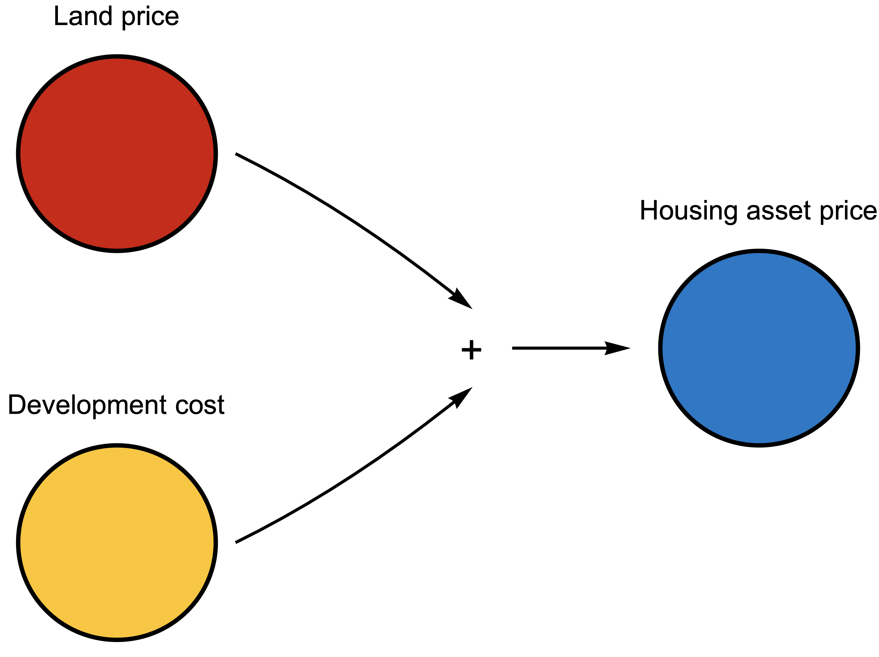
The image below shows the commonly assumed causality that the asset price of a home is caused by the summation of the land price and development cost. It is true that this equation generally holds: Land price + Development cost = Housing asset price.
But this is not the way causality flows. We know this because we must first ask, “Where does the land price come from?”
Land can’t be independently priced. Its value is derived from its possible uses. Land is akin to a financial derivative. It has no value apart from its ability to be combined with development costs to get an income-producing asset (or, in the language of derivatives, an underlying asset), in this case, a house.
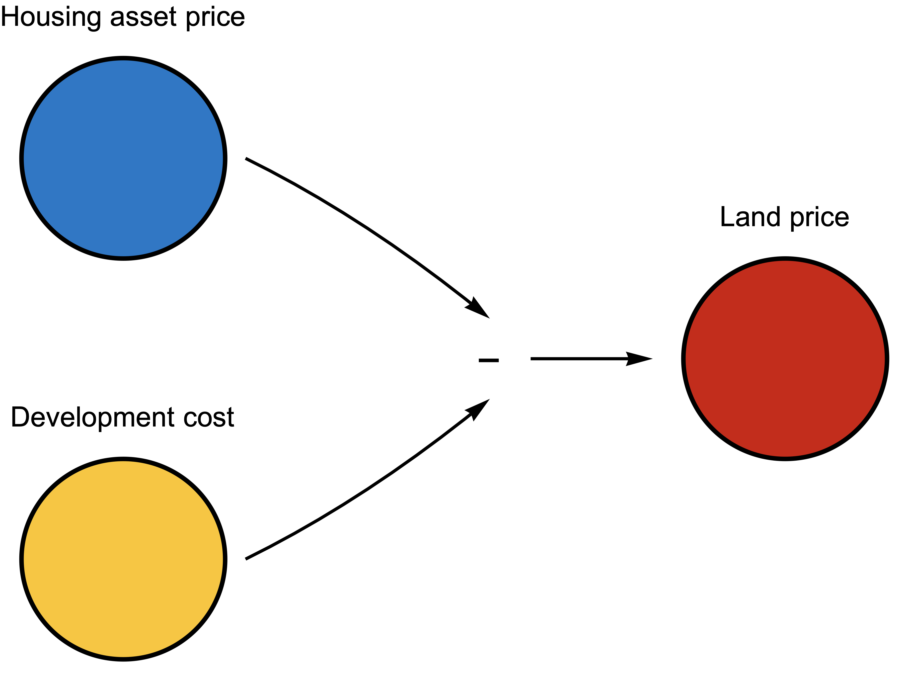
The value of any financial derivative is caused by the value of the underlying asset (the house) minus the strike price (the development cost). Or in other words, the value of land is the housing asset price minus development costs. That’s the way causality works: Housing asset price – Development cost = Land price. Land is a residual. It is what is left over to fill the gap to make the equation hold, as I’ve shown below.
The values of land and development add up to housing prices not in a causal way, but because market equilibrium forces sustain these values.
It is exactly the same force that prices housing assets based on relative returns to other assets in the economy—there is an arbitrage opportunity if these values don’t add up.
I explain this in my book, The Great Housing Hijack, as follows.
Consider the case where the price of land is $300,000 per developable lot, and the cost of developing a home is $300,000, but the price of a home is $500,000. No one will buy the land at the $300,000 price. Why would they? If they did, they would be paying $600,000 to buy land and build a home that would be worth $500,000. The price of the vacant property must adjust back to $200,000 so that the cost of buying an existing home, or building a new one, is the same.
The opposite adjustment would happen if a plot of land was priced at $100,000 and the cost of building a home was $300,000, while the price of existing substitute homes was $500,000. This situation can’t be sustained either. Why would the landowner sell for $100,000 when they could take two assets—the $100,000 of land and $300,000 of cash to build a home—and combine them to create an asset worth $500,000, pocketing the $100,000 difference?
This equilibrium market pressure doesn’t mean that all transactions are perfectly priced. These asset swaps of cash for construction are risky and take time. That’s why there are margins built into the development cost at all steps along the way. But these margins won’t always cover costs—the nature of risk is the unexpected variation. So some housing developers will go broke trying to make this arbitrage, and others will earn more than their expected margin.
This is exactly how financial derivatives are priced.
If you have a financial derivative that gives you the right to buy a share in BHP at a strike price of $30, and that share is currently trading at $50, the derivative asset (an option in this case) is worth $20. The price of the derivative does not cause the price of the BHP share, but it is the case that the derivative (like land) is worth exactly the value of the underlying BHP share asset (like a house) minus the strike price (like development cost).
The price of housing assets is determined in the same way as all assets, based on the arbitrage of returns and risks. The value of land for housing is priced the same way as a financial derivative that doesn’t directly produce income until it is transformed into the underlying asset. We must remember this asset pricing reality before looking at the physical characteristics of housing to explain its pricing.
Construction cost determines the optimal project, not the price
Are lower (higher) land values the only effect of the development cost of a home being higher (lower) than it might otherwise be due to things like fees and charges, higher construction costs due to regulatory requirements, or any other reason?
That initially seems the case.
In our previous example, if we add a $50,000 fee to the $300,000 development cost, then at a market price of housing of $500,000, the land value would be $150,000. If we remove that fee, the land value would rise back to $200,000.
But there is more to it.
When the cost to transform land into one use change, it can also change which project generates the highest value. That includes non-housing uses being the highest value use, and is why people say things like “these fees and charges have rendered housing development infeasible.”
The development cost for transforming land into housing affects the location, density, and quality, or what I would label the shape, of the pool of feasible development sites.
Let me repeat.
If the cost of developing housing increases, then the pool of feasible sites will shrink, both across locations, in terms of the housing density at each location, and the optimal quality or size of each dwelling. If development costs decrease, this pool of feasible sites will grow, both in density, quality, and across locations.
Before I explain how, I must first explain that just because a location is feasible today to develop new housing, that doesn’t mean it will quickly become new housing. The rate at which new housing is built out of the pool of feasible sites is also regulated by market conditions, where the market equilibrium is that the rate of return from waiting equals the rate of return from developing now (this article is recommended reading on this concept).
This is why the pool of feasible sites is generally many times larger than the rate at which homes are developed per year, perhaps 20 to 100 times larger. A town that has a market rate of new housing production of 1,000 homes in a year may have locations where housing is presently feasible for 100,000 dwellings. In South-East Queensland, if we narrow this pool to only a small fraction of those sites whose owners already sought and received planning approval for new apartments, we get a sub-pool of 115,000 approved new apartment dwellings, with only 7,000 developed per year.
What I am referring to with the idea of shaping the pool of feasible sites is where and how dense this very large pool is.2 Out of this pool, it can always be more feasible to develop tomorrow, next year, or in a decade. Markets don’t build tomorrow’s homes today.
Yet the Productivity Commission report assumes that feasible homes are instantly built and that house prices are due to the sum of land and development cost, getting causality backwards. This leads to the strange idea that lower construction prices will mechanically lower housing asset prices by an equal amount and completely misses the true choices of property owners over the density, quality and timing of new housing investment.
Feasibility and the highest value use
Whether housing is feasible depends on the value of land for some housing option exceeding the value for other uses, such as industrial, agricultural, commercial, or any other alternative that is allowable.
Feasible housing means that the land value, arising from a housing project’s developed asset price minus development cost (as we discussed above), is higher than the land value for the property’s current use, such as agriculture, industrial, or any other.
Yet even if there is a feasible housing project, it doesn’t imply that any housing project is feasible at that location. There will be many housing alternatives that are infeasible and many that are feasible.
Let’s use an example.
Say you have an 800 sqm block of land on the fringe of a regional town where any type of housing is allowed to be built. Here are some of the options you might have to develop that block into housing. The dotted cells represent the idea that this list of options can extend in either direction in terms of housing density—we aren’t limited to just six possible projects.
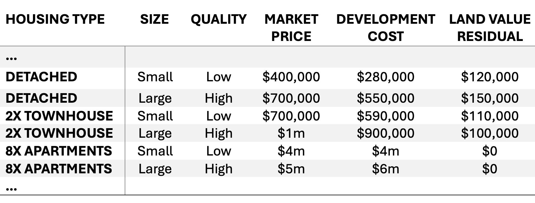
It might seem weird to put eight high-quality large apartments as a development option at this location, but the planning regulations allow it. It just happens to be that a $625,000 market price of an apartment at that location (so that the block of eight is worth $5m) is lower than the development cost of $750,000 per apartment (or a $6m total cost).
Does that mean that apartments at this location must soon be worth at least $750,000 because development cost causes market prices?
No.
It simply means that this type of development is infeasible at this point in time at this location. Development costs cannot affect housing prices, or we face the irrational conclusion that any housing development alternative must always be feasible.
Let’s continue this example by noting that at this location, the highest non-residential use (e.g. farming) has a land value of $95,000. In this scenario, the townhouses and detached house projects alternatives are all in the pool of feasible housing at this site, meaning that the value of the land for this residential use is higher than the value for the non-residential use, but none of the apartment alternatives are.
But wait!
Let’s add another complication to this scenario. Imagine now that the local council has realised that the cost to service new homes with public infrastructure is about $15,000 per new home and has decided that instead of sharing that cost amongst existing residents, this cost will be added upfront as a fee on new housing which they hope properly prices the full development cost of a new home.
Now, what happens to our land values across the residential project options?
We can see on the table below that this makes two townhouse options infeasible at prevailing market prices relative to non-residential uses which value the land at $95,000.
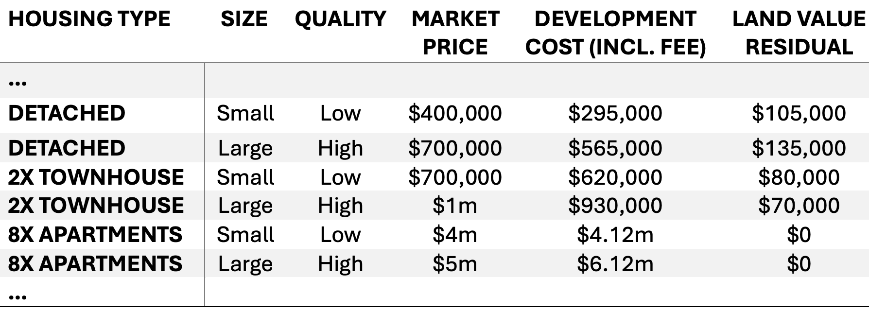
We have shaped the pool of feasible options at this site, even though the option with the highest land value residual is unchanged.
It could be the case that this site is rendered completely infeasible for all housing options with a fee of $55,000 per dwelling. That would make even the large detached house project less valuable than the property’s current agricultural use. That would eliminate this site from the pool of feasible housing at the present time.
It is normal for some locations on the fringes of urban areas or those with high value alternatives to go from feasible for some type of housing, to infeasible and back. This happens due to rising and falling housing prices, rising and falling construction and development costs, or changes in the value of non-housing uses. The shape of the pool of feasible housing changes predominantly due to market conditions.
Another subtle effect of higher development costs is to re-order the land value residual of different housing project alternatives. In other words, variations in construction costs can change which housing project is the one with the highest value on a site.
Density, quality, and development cost
We have shown that the idea that the sum of land value and development costs causes the market price of housing has causality backwards. We have also shown that out of all the possible projects on a site, it is the one with the highest land value residual that determines the value of land, even though many alternative residential projects can be feasible at any point in time.
The idea that there is not one but many alternative feasible projects helps us to see a general principle about how development cost affects the choice of project density and quality. This is the main missing bit of economics in the PC report.
Higher construction costs relative to market prices for homes lead property owners to economise on construction by building lower density (and quality) at the same locations.
The reason for this is that there are diseconomies to higher-density development.
The construction cost for the same apartment in a 50-storey building will be higher than in a 20-storey building. This is why we don’t build tall buildings in low-value locations.
This principle is a general one and applies to low-density housing types like detached homes and townhouses. Townhouses are generally only feasible in higher value locations than where detached homes might first be feasible above non-housing uses.
Because most of the public debate about town planning regulations involves situations where regulations limit density below what would otherwise be built at a location (usually a high-value location), it is common to think that more density always gives a property owner a higher financial return from development. But it is just a quirk of the interaction of planning regulations and market forces that regulations can only restrain density and limit property owner returns, but can’t require higher densities that would also limit returns in the same way.
Diseconomies of density mean that any property owner will consider from the pool of projects those with increasing density until such time as the marginal cost of more density equals the price they get for that extra density. Then they stop. This is how a property owner determines which project maximises the land value residual out of all the different density project options.3 The chart below demonstrates this.
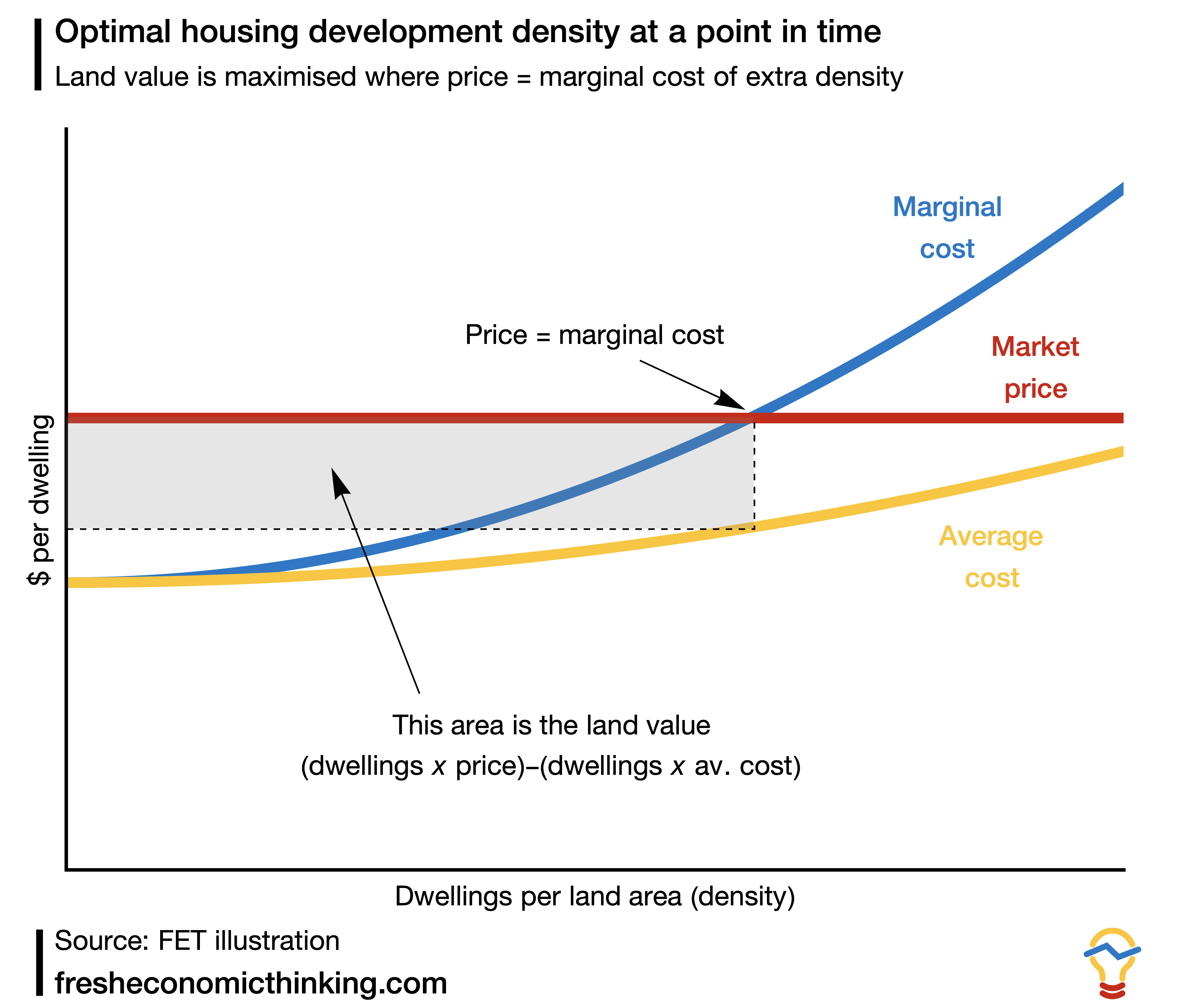
Here, the marginal cost (meaning extra cost of building more densely) rises faster than the average cost of building a dwelling, as it must when there are diseconomies of density.
Although all the densities where the average cost is below the market price might be feasible (i.e. all densities shown in this range), the density that will provide the highest value to the property owner is where price equals marginal cost. This density maximises the area of the rectangle between the total revenue (market price multiplied by number of dwellings) and the total development cost (average cost multiplied by the number of dwellings).
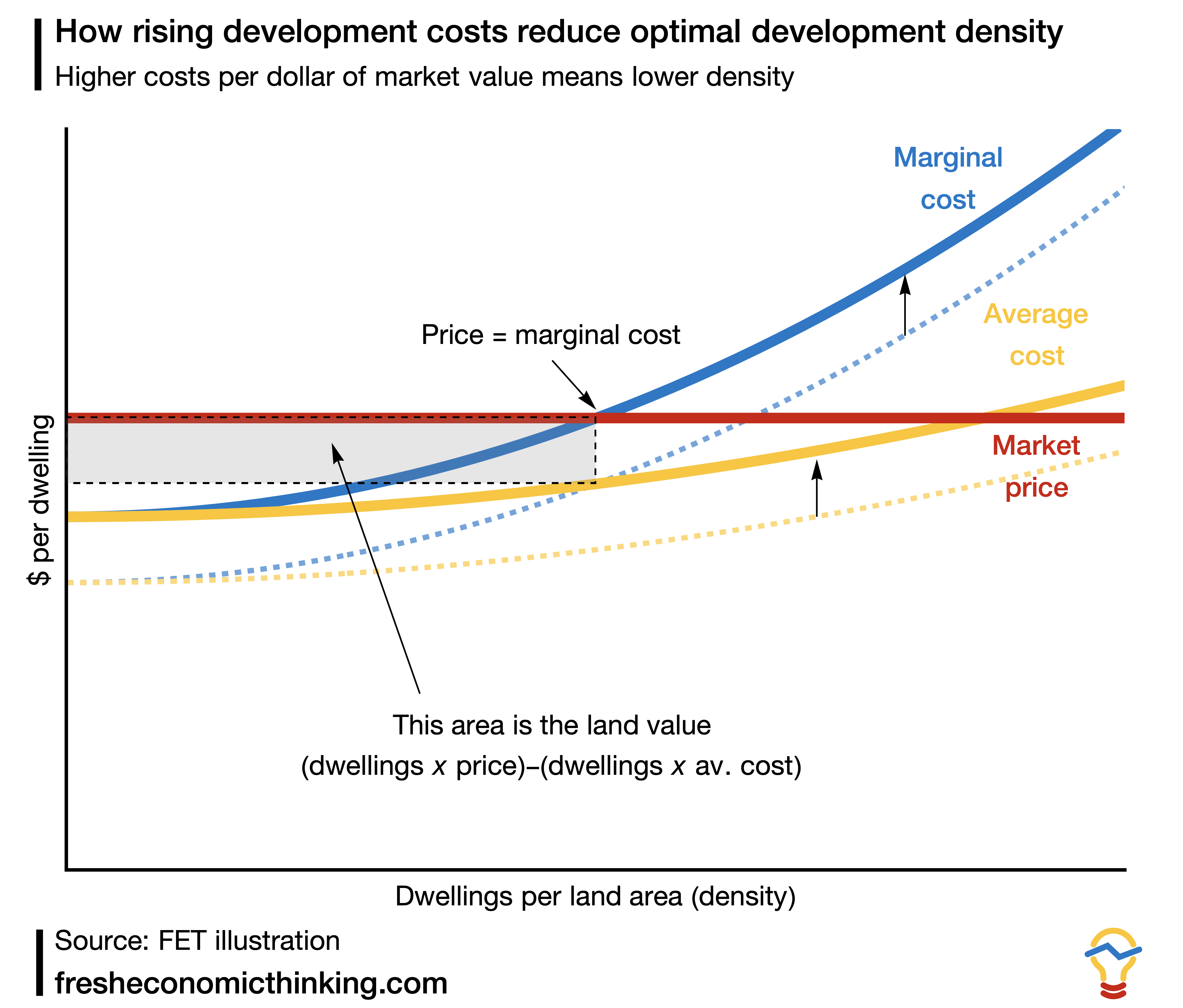
What happens if we now add costs per dwelling to this project, such that the average and marginal costs rise by a fixed amount per dwelling? This could be due to things like higher construction costs (because of a lack of productivity), or due to new fees and charges on housing development.
In this scenario, both curves shift upwards, shifting the point where price equals marginal cost to a much lower density. Land value is still being maximised when it comes to the choice of projects, but the land value has fallen more than in proportion to the added cost.
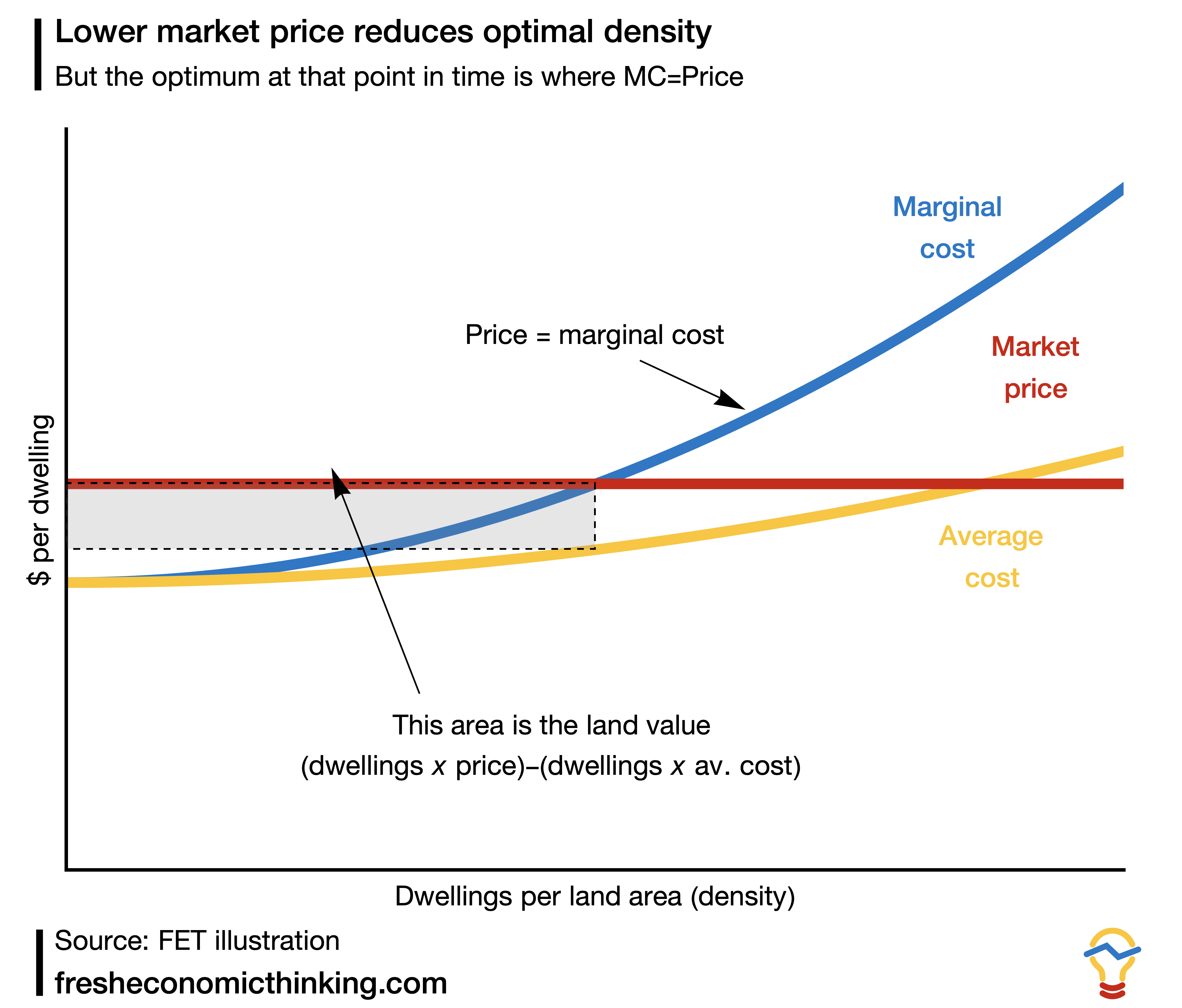
The same effect of declining optimal density happens when market prices fall, as the image below shows (which is why I have said before that we are at the tax breaks stage of the property cycle). Of course, the reverse holds too, so that rising market prices and falling development costs increase optimal density.
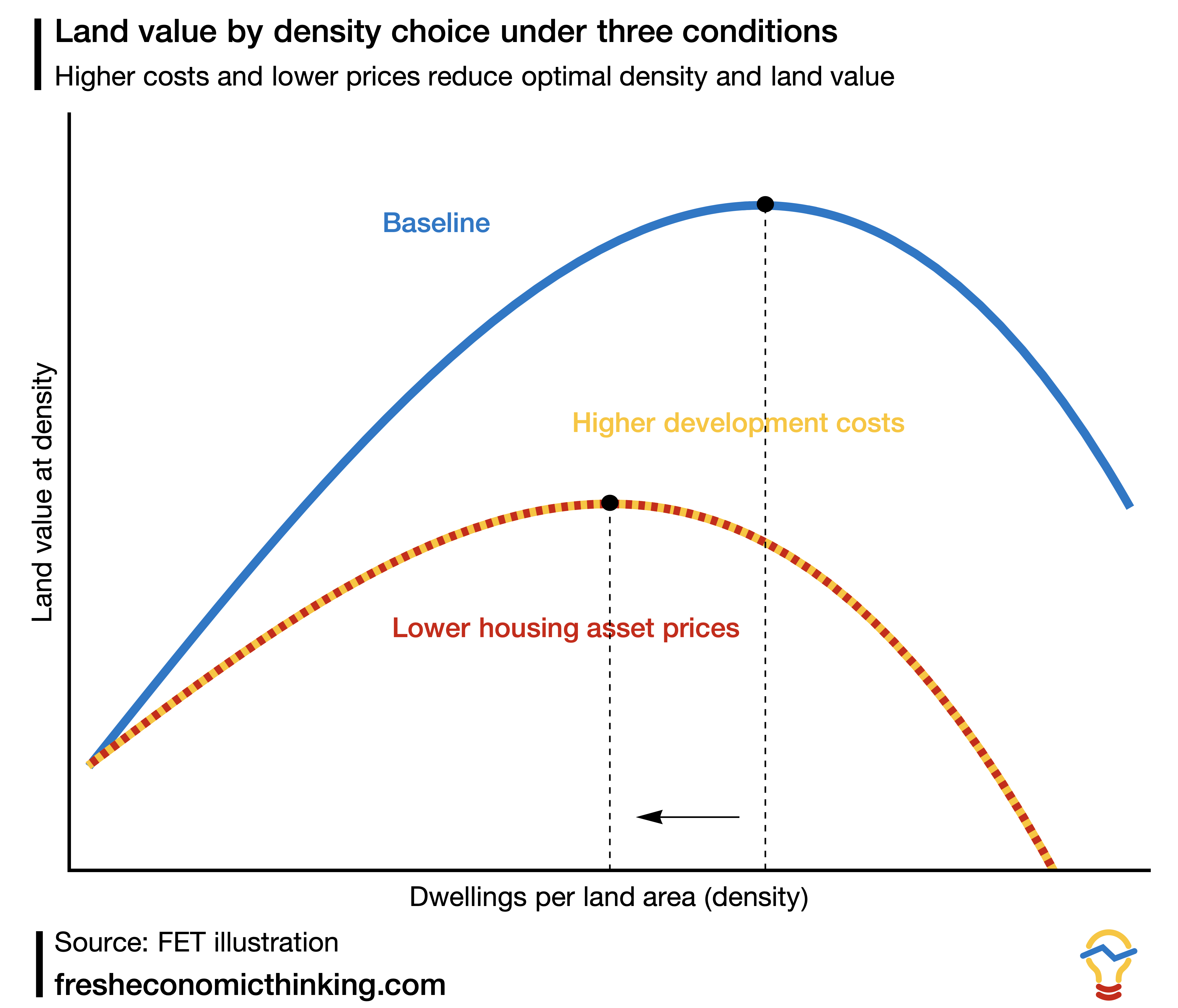
Another way to look at this exercise of finding the optimal density and seeing the effect of either higher development costs or lower housing asset prices is to plot the residual land value at each density choice. We see below this approach applying the residual land value calculation to all possible density choices for given costs and market prices in the previous examples. Higher development costs and lower asset prices have the same effect on reducing land values and reducing the density of development that maximises land value at the time of development.
This economic relationship between development cost, price, and optimal density is the reason that tall buildings are only economically justified in high-value locations, and also why the tallest buildings in a city are usually proposed at the peak of the housing asset price cycle.4
It is also worth noting that this relationship is all about relative development costs and price. High value locations typically have higher development costs, which also limits the optimal density, while low value locations have lower costs, allowing density that would be uneconomical if that area faced the same high development costs as in high value locations.
While density is a very important dimension of project choice, it is still just one dimension over which projects are optimised. As our previous example tables showed, there are also quality dimensions to projects. And as luck would have it, the same economics applies to these quality dimensions too—does the extra price received for adding marginal quality improvements exceed the marginal cost of building them? If so, keep adding more quality.
This quality might be in the form of more bathrooms per dwelling (keep adding bathrooms to designs if buyers pay a premium that exceeds the extra cost of the bathroom), carparks, quality of interior finishes, external design, or any other feature.
The fact that property owners must choose what project works best across many dimensions to squeeze the most out of the prevailing market price is why property experts have such a crucial role. Choosing what projects work where, when to build them, and how to optimise across every aspect, from bathrooms to car parks, to quality of finishes, given market conditions, makes all the difference.
Showing how the optimal project choice and density will change in response to market price and development cost changes helps us better interpret claims from the property industry that “these charges make our project unviable” or “we can’t make the project pencil in this market”. Often, these more specifically mean “we can’t make the optimal project under previous conditions work, and we don’t want to build the currently optimal project because it will make us less money, even though that project is still feasible.”
We have an interesting scenario now in Australia where overall construction costs have recently risen, but the market value of extra quality has increased. The logical response to these conditions is to decrease density but increase quality to find an alternative project that maximises the residual land value.
Two examples from my neighbourhood show this logical response in action.
First, there is an apartment project that was approved for 145 apartments (1, 2 and 3 bed). In the face of higher development costs, the developer modified their design to be just 44 luxury apartments.
Second, this nearby project scaled back its density from about 440 approved apartments to 164 luxury apartments and townhouses, going for extra quality and amenity with much lower construction costs.
To reiterate, the cost of development shapes the pool of feasible projects across sites, and can change which project out of the pool of feasible ones is the highest value project. As the construction cost rises, the market will economise on construction by building at lower densities, given the same market values.
The rate of production vs the pool of feasible sites
Will property owners slow down development as well because the shape of the pool of feasible housing is lower density? That all depends on the market conditions.
Markets will always delay building feasible new homes. This is not because of the personality of property owners or their evil nature, it is just that the market selects for the most patient and most optimising property owners, and those property owners pay the most for the site and optimise over time as well as density, quality, as we have discussed.
As a quick summary, the asset market equilibrium will mean that the rate of return on a dollar invested in holding a feasible site and not building housing will equal the rate of return on developing it. The absorption rate, or the rate of new housing development, is the rate at which trades are made, or cash for new housing development, to maintain this asset pricing equilibrium. It is possible to have a fast absorption rate of new housing at low or high density, and low or high prices relative to development costs.
What affects the pace of development from the cost side is the rate of change of development costs, not the level, as this is what changes the trade-off to waiting. Rising costs will generate an incentive to delay, and falling costs will accelerate development. But it is possible to have high and falling costs, or low and rising costs.
Rather than make this article a lot longer, I will direct the curious reader here:

Putting the PC results into context
Let’s put all this together now in the context of the Productivity Commission's claim that low productivity in housing construction leads to higher development costs, slower housing investment, and higher housing asset prices.
First, as I showed in Part I, we don’t know if productivity has increased or declined based on the analysis undertaken. Construction costs can rise with an increase in measured labour productivity or fall with a decline in labour productivity. We also know that higher density housing has higher construction costs for the same value of dwelling, even though high density housing usually has higher measured labour productivity.
A big part of why the PC’s analysis can’t determine what they are claiming is that when construction inputs see gains in labour productivity due to mass production or prefabrication, those activities get reclassified as manufacturing, leaving the construction industry looking like a productivity laggard.
Even then, the proportion of the value of a housing asset that is related to the construction cost component analysed by the PC is surprisingly low and could not sensibly lead to the strong conclusions they made.
We have just examined how markets price housing assets and land, and how property owners optimise the choice of housing projects to maximise the residual land value out of the choice of many projects of different densities and qualities in the pool of feasible homes.
With this bigger picture asset pricing context, we can revisit what the PC did.
They looked at a $37 billion component of the value added in housing construction nationally and divided that number by the number of workers involved in those construction services.
Since around 40% of housing construction goes to renovations and maintenance of the existing stock of 11 million homes, in terms of building new homes only, we are left with about $22 billion of the value of new homes in the PC’s labour productivity assessment.
With about 180,000 new homes completed with a market value of $180 billion, we are looking at measured labour productivity of a component that reflects only about 12% of the market price of a new home. A tiny fraction.
I’ve created the diagram below to help provide some bigger context. It shows the market price of a typical new home and the component values, zooming out from construction to development, which includes land price, margins for risk, and other non-construction development costs.
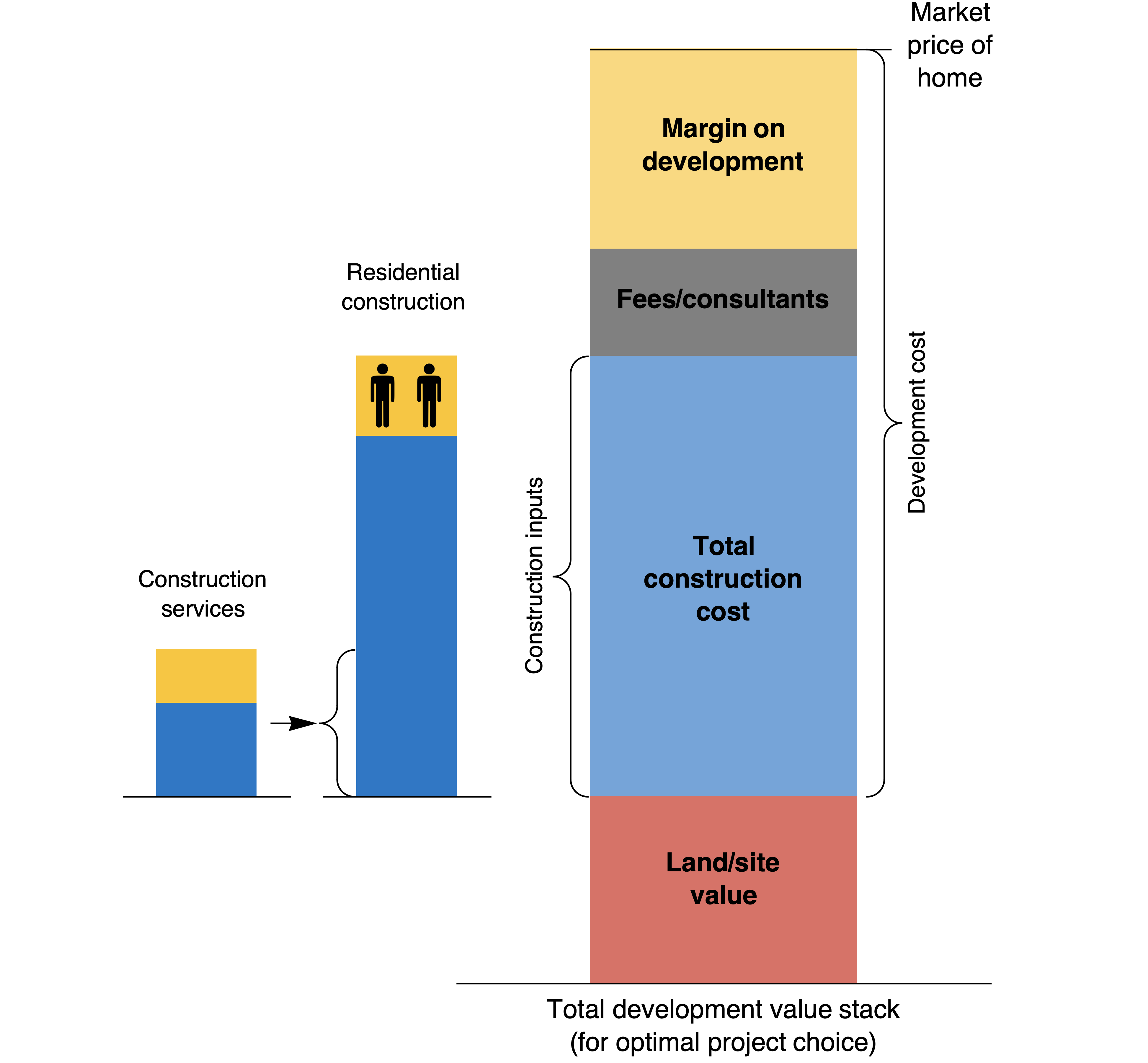
Remember that the asset price is not caused by the sum of the value of these components. The most profitable density and quality of projects are chosen to maximise the land value part of the value stack, given market prices and development costs.
Out of the construction cost component, which is shown here as 40% of the value of a new home, the PC looked at the productivity of just 30% of that component (the yellow parts of the two left bars of construction services and residential construction), which is how we get to the 12% of total asset value of new homes being the Gross Value Added (GVA) used in their analysis (30% x 40% = 12%).
Not only have we learnt how housing asset prices are determined, how the projects with the highest land value residual are chosen from the pool of feasible ones, both by density, quality, and across time, we have now put the scale of the PC’s analysis in the context of these greater market forces.
Here’s what you must believe to buy the PC’s story of housing construction labour productivity leading to higher housing asset prices.
First, you must believe that the empirical approach to measuring construction labour productivity is valid. Part I explained in detail how the analysis undertaken missed some critical economic insights, and why simply looking at price changes is probably the better approach to understanding if gains are being made in sub-sector productivity.
Second, you must believe that this labour productivity decline is causing higher construction costs on a like-for-like project. Again, Part I shows how we can’t know that, and here in Part II, we have shown that higher density housing, while generally high on measured labour productivity, has higher construction costs per comparable (i.e. same market price) dwelling.
Third, you must believe that causality flows from development costs (which include construction) and land price to asset values, which is the opposite of what we now know.
Fourth, you must believe that projects cannot change density and quality in response to changing construction costs, nor does the market optimally choose the timing of new housing development.
Once you believe all that, you have a 12% decline in construction labour productivity over 18 years of a component that makes up, on average, 12% of the value of a new home. Taking productivity declines as the inverse of construction cost increases, we get at most a 1.4% asset price effect over nearly two decades, even if we believe all of these unrealistic assumptions.
Even if you take the most generous assumption that it is the labour productivity decline relative to the economy average that matters, we have a 40% relative decline in 12% of the value of a new home, giving us a 4.8% asset price effect since the mid-1990s.
So what?
Let me wrap up as best as I can about the right way to think about housing markets and housing asset prices, and reiterate why I am so frustrated with the PC report and subsequent commentary.
I apologise that there is a lot in this, and if it's your first time reading this type of detail on asset prices, land valuation, and so on, it will be difficult to follow.
First, asset prices arise due to the same factors as every other asset: risk and return. That’s because people can swap a housing asset for any other asset in the economy at any time.
This asset pricing mechanism is also why it always appears that the market price of a new home is the sum of the land price and the development cost. This is not a causal sum, but an equilibrium outcome. It must be the case that these are equal, or someone is going to make free money. What adjusts to maintain this equilibrium is the price of the land.
Second, every site can be used for many feasible alternative housing projects, not just one. These projects vary by density and quality. In general, higher density projects have higher construction costs (diseconomies of density) for the same value of home built. Variation in construction cost will mainly vary what the optimal density (and quality) of a project is at a given market price at a point in time. A much more subtle effect is how changes in construction cost can affect timing decisions.
It can be the case that planning regulations that limit density result in new homes with a lower construction cost on average at those locations because of diseconomies of density.
Productivity gains in housing construction are not taken in the form of lower prices at the same density and quality. This is what the historical record shows. They are taken in the form of higher density and quality, and in the form of higher incomes across all economic sectors due to the interactions Baumol is famous for identifying.
Lastly, even if you ignore all this and take the PC story of declining labour productivity and higher housing asset prices as a causal one, which is wrong, it at most explains a 4.8% relative rise in the asset price of housing since the mid-1990s.
None of this is to say that we shouldn’t promote productivity in housing construction and its manufacturing inputs. We should. However, any such gains will not only affect housing markets but will be felt across the economy through the many adjustments that must arise, ending up as a general rise in real incomes, exactly as William Baumol describes, rather than in lower housing asset prices.
A credence good is the name economists give to a type of product where the buyer cannot know the quality in advance, nor can the quality be known after the good is consumed. Think of a surgery or medical treatment. We don’t know if it’s right for us, and we often still don’t know after the fact. If a builder constructs my home, I can’t not know whether they did a good job beforehand, but most buyers can’t know themselves afterwards either, relying on various approaches such as third-party inspectors to resolve this information problem. Generally, this information problem is why there are much stricter rules on single house construction rather than more commercial apartment construction—buyers of apartment construction services are expected to be in the best position to judge the quality, more so than any independent inspector.
It is true that in some locations, suburbs or even towns, this pool is relatively small. However, substitute towns do take up the market for new homes—every location is a substitute at the right price. One example in Queensland is Noosa, which is a small coastal council area north of Brisbane. Here, the pool of feasible sites is very low. But in neighbouring coastal areas, the pool is very large. This whole market is a substitute, and the fact that Noosa restricted its pool shaped where development happens in the broader region, without necessarily leading to fewer new homes per year developed across the region.
You can simply calculate the residual land value for each project with increasing density and pick the one that maximises that value. The marginal approach does the same thing by looking at slopes.