Explainer: Markets efficiently delay building feasible new homes

Some people LOVE that markets make trade-offs but HATE when markets make inter-temporal trade-offs. Let's go deep into the economics of why housing markets build faster or slower.

---

Note: Monthly FET subscription prices are rising for new subscribers. This is intentionally to make an annual subscription much more attractive. Current monthly paid FET subscribers are unaffected and will always keep their original price. Yearly prices remain unchanged.

I hope you find it in you to support my efforts here to raise the quality of our economic conversation with an annual subscription (it might even be tax deductible for you!)

---

Markets are good at making trade-offs.

Even if everyone in the market is irrational, the constraints of the system—of money balances and property rights—often lead to acceptable and favourable trade-offs.

I explained that logic in more detail here.

Markets also encourage innovation because new technology can break down old trade-offs by getting more output (in terms of its value to others in the economy) per input.

The market in real estate is no different.

This market efficiently uses high-value locations for high-value uses. This means people with a low value for a location will be excluded from that location. It is the same in other markets. Those who place a low value on luxury goods won’t buy them.

You might claim this is often because of unequal wealth and income. And you would be right. Some people don’t like the inevitable inequalities in market outcomes, and they often search for market failures to explain it, especially in real estate markets (as I document in this academic article).

Today’s topic is not inequality.

The topic today is the forgotten temporal dimension of the trade-off that participants make in all markets. As well as allocating products to who values them most, markets allocate across time to when new products are valued most. In other words, markets will efficiently delay or bring forward production decisions across time.

For example, Toyota is bringing its new Prado model to Australia this year. But it isn’t pricing them to maximise its 2024 profits only, even though the market for four-wheel-drives in Australia is very competitive and lower pricing could greatly increase 2024 sales. Toyota is pricing in a way that it expects will maximise not just its 2024 profit (quantity of sales in 2024 times the margin per vehicle) but the present value of its flow of profits in 2024, 2025, and beyond. Toyota will bring forward sales with lower prices only if it increases the total present value of production profits by more than it gives up in future sales at higher prices.

All firms are forward-looking and consider the effect of their choice of production rate and pricing on their future profitability—not just this year’s, this month’s or this week’s profit.

Back in 1931, a popular concern was that markets would use up natural resources like coal, minerals and oil, too quickly. Were markets just wasting these resources? Harold Hotelling pondered that question and explained how (like Eric Crampton explained more recently) markets won’t inefficiently use up resources too quickly. They trade off extracting more resources now with extracting more later.

Unfortunately, most economic analysis mostly assumes away the intertemporal trade-off, and this can lead to major errors in reasoning and interpretation of evidence.

This intertemporal trade-off in real estate means that most feasible housing development projects are delayed into the future, even when prices or rents appear to be high and projects are profitable today.

As I noted earlier, some people don’t like this inevitable market outcome, so they search for market failures to explain it. But it’s not a failure. We want markets to efficiently delay building homes, don’t we?

Why isn’t this well-known?

I admit that it took me a while to notice intertemporal trade-offs and fully recognise their significance. That’s probably because most economic analysis at best consists of assuming away time altogether, simplifying to a short-run (single static period) and a long-run (some other single static period) with no way of bridging the two.

Because economists are trained this way, it leads to a blind spot across the discipline when it comes to timing decisions.

On X, I was surprised to see that a seemingly innocuous post below garnered over six million views in a few days. It simply asked why landowners in private markets would build so quickly that prices fell.

Which is a very good question!

The thousands of replies almost unanimously explained most smugly the crossed swords of supply and demand from Economics 101 that they learnt, forgetting that this simplified model assumes away the time dimension.¹

The replies showed complete ignorance of the dynamics of housing supply and price effects from supply today on profits tomorrow— a hot topic of study in the academic literature with many researchers trying hard to understand it.

People for some reason don’t believe me. They want settled science—preferably ECON101.

So today’s article is a deep dive into the forgotten economics of inter-temporal market trade-offs when it comes to housing production. It takes you far beyond ECON101 and to the cutting edge of knowledge about when and why homes are built.

Let’s start with a quote from urban economist Alvin Murphy, who noted in a working paper version of his 2018 paper entitled A Dynamic Model of Housing Supply that:

A static model would predict that a parcel owner would build the first time it becomes profitable, whereas the dynamic model allows a parcel owner to delay building (even when profitable) in order to attain higher profits at a future date. [p15]

That line didn’t make it into the final version of the article, which in typical economics fashion was published eight years later,² but that version makes the same point clearly in its opening sections.

In the model, landowners choose both the optimal timing of and the optimal size of construction. These owners take into account current profits and expectations about future profits, balancing expected future prices against expected future costs. Analyzing these decisions with a dynamic framework allows one to meaningfully separate the effects of current profits on supply from the effects of expected future profits on supply, which is the key mechanism through which forward-looking behavior reduces the housing supply elasticity.

Here’s more

Forward-looking behavior substantially reduces the responsiveness of landowners to current price changes. This reduction occurs because rising prices make building today more attractive, but also signal higher future prices, making waiting more attractive, thus reducing the responsiveness to current price. Interestingly, this forward-looking behavior suppresses the responsiveness to current price by a much greater extent during boom periods with rapidly rising land and house prices.

That forward-looking behaviour considers the returns given up on the assets required to develop new homes (the cash to pay for construction and the land asset) for the returns to the new home (net rent and capital gain) after consideration of local price effects from faster development.

A simple demonstration

The tools most relevant for understanding intertemporal trade-offs come from a field of economics known as real options, which analyses timing choices of irreversible capital investment—clearly relevant for understanding housing production.

The logic of real options and the intertemporal trade-off means that for new housing, two conditions must hold to make it worthwhile to build a dwelling today rather than tomorrow (though not really today or tomorrow, it could be this year instead of many years in that future or any other trade-off between some future period and the present).

These are:

1. The market value of a dwelling must equal the development cost plus the value of the land (which itself gets a value because it is a financial derivative—an option). In the lingo of real options analysis, this is called the value matching condition.

2. The total return to the developed home must equal the total return to the assets swapped for it. In the lingo of real options analysis, this is called the smooth pasting condition.

The first of these is a bit tricky to understand if you have in mind that the price of goods comes from the summation of input costs, but the second is more important for dynamics and I think it is quite straightforward to grasp.

Value matching

It seems intuitive that new homes only get built if the market price of what is built is as high as the market price of the land plus the development cost.

Where property markets differ from many other markets is that homes need places to put them, and those property rights to places, or land, have a value because of their potential ability to generate future returns. Land gets its value like any other financial derivative.

So the important thing to understand is that there are market constraints on being able to buy land cheaply, then build homes, and make abnormal profits (i.e. profits that more than compensate for the risk involved in that process).

The reason is that every potential land seller also has the option to build homes themselves and take that risk and make a profit. They can arbitrage the value themselves. So the sale price of developable land, at a minimum, will be the residual of the market price of developed housing, minus development cost (which includes a margin for the risks involved in actual construction and sale).

The diagram below shows on the left the market price of a completed housing project. The next part of the diagram has the land value (yellow) as the residual of market price minus development cost (blue) at the value-matching equilibrium condition where development today is the highest value option for the land.

Let’s make this example more concrete. Imagine that a home is worth $1 million (for the sake of round numbers). By definition, if the home costs $500,000 in construction and development costs (including a risk margin), which is the blue bar, then the land is worth a minimum of $500,000, which is the yellow bar. The sum of these inputs equals the market price, but only because the land value is caused by the market price of the home minus the development cost.

The value matching condition says that this must hold for the marginal project that will be built today rather than delayed until tomorrow.

But what is commonly misunderstood is that a land value of housing price minus development cost is the minimum amount that land will be worth for a development site.

It might be the case that at a particular location for a particular lot, buyers are willing to pay $600,000 for the lot, even though construction and development costs (including a risk margin) are $500,000 and homes are only worth $1 million.

The land is valued more highly than the residual for the best choice project today because the land owner has the option to instead build a different project later that might be even more valuable.

The next columns in our diagram show this common situation where there is a delay premium in the market value of land. That extra value of land above the residual value, if developed today, is an option premium. This premium is the value the owners (buyers and sellers) of land derive from being able to choose when to develop and potentially build something bigger, better, and more profitable in the future on that site. In this case, landowners think there are more gains from waiting.

So we have seen how land values can be above the residual of today’s housing price minus development cost because of an option premium. But why is the value matching condition a minimum land value for a site with development potential?

The far right of our diagram shows a hypothetical situation where the market value of land is lower than this residual value matching condition. The trick to understanding why this situation cannot happen is because it requires land sellers to leave money on the table—after all, they have the option to develop or delay if they want to.

It can’t be the case that land is available to buy in the market for $400,000 if homes that cost $500,000 to build (including a margin for risk) are selling for $1 million. Sellers are giving up $100,000 if they sell the land rather than building a home and selling it themselves. So they won’t accept a lower price.

In asset markets, the concept of “price is above cost” doesn’t work. How does that apply to shares (stocks) in BHP or Apple? How can the price of those shares be above their cost? The price is the cost. The same applies to land.

It is a common mistake to think that land can be purchased at a price that represents its value only if the current use is allowed. People say things like “Only zoning is stopping developers from buying land at agricultural prices and building homes”.

That’s not how land markets work.

If you are allowed to build homes, no property owner will sell the land for the agricultural price, and you will be competing with other buyers willing to pay at least the residual value of the price of development today minus the cost.

So to wrap up, the value matching condition means that for the marginal site that could be built today (with the lowest value to delay), its value is equal to the residual of the market price minus the development cost. For other non-marginal development sites, the land value is above this residual of today’s market price for homes minus development cost.

But even if this value matching condition holds, it is not enough to justify new housing production today. The second condition must hold too.

Smooth pasting

Building a new home is an asset swap of cash and land for housing. That swap will only occur if the expected rate of return is higher for the purchased asset than the asset given up to get it.

Not only do the sum of values of the land and cash (for development costs) assets given up to build a housing asset have to match (the value matching condition), but so do the rates of return on the assets given up have to match the rate of return on the new housing asset.

The rate of return between building a home and not building will be equal in an inter-temporal market equilibrium.

The diagram below shows this second equilibrium condition, known as the smooth pasting condition (or sometimes it is called rate of return equalisation). The left in red shows the total return from one period to the next for developed housing, represented as the rate of change in total value (including net rents and capital gains).

So if the $1 million home in our hypothetical example makes $60,000 in capital gains and net rental income, then that’s a 6% total return— the value of that asset in a year’s time is $1.06 million.

The next part of the diagram shows the return to waiting from the gains in value to the land (yellow) and the return on cash needed for construction (blue). Here, we have a case where the capital gains to holding developable land are 6% and the interest rate on cash is 6% too.

In this situation, the rate of return from waiting is equal to the rate of return from building. If you had $1 million in a home your assets would be worth $1.06 million next year, and if you had $1 million in cash and undeveloped land, then your assets would be $1.06 million in a year’s time as well.

On the right of the diagram is the situation where the rate of return from waiting is higher than from having a home. Say the interest on cash is 7% and the value of developable land is growing at 8%. In this situation, you give up $1 million of cash and land assets making $75,000 in total returns to get a $1 million house asset earning $60,000 in returns. You will be better off in this case by waiting instead.

People always forget the smooth pasting condition that must apply in a housing production equilibrium.

Back to the rate of home production (i.e. supply)

Let’s check in. We have two dynamic equilibrium conditions that must hold in a housing production market equilibrium.

These conditions help explain why most feasible sites for housing remain undeveloped — the market is trading these homes into the future, efficiently delaying them until they are produced at the most valuable time. If the rate of return to waiting to build a home is higher than from building it now, then markets are efficiently delaying housing production.

But how do we know how many homes are built each period? Where does that rate of housing production come from?

There must be a flow of new housing per period that sustains these equilibrium conditions.

We need to think about this carefully.

And to be clear, we are now approaching the end of our collective knowledge about what determines the rate of housing production.

There are many possible trades of assets in housing markets. For example, you can trade cash directly for homes, as well as trading cash for construction and combining that with a land asset to get a home. You can also “cash out” land and get its value as cash by selling rather than building homes.

The available trades are shown below. In each of these asset swap markets, equilibrium forces dictate the rate of trading, which depends on the relative returns to each asset.³

The diagram also helps us understand why construction cycles tend to track house price cycles. If you have cash and want to get the return from homes instead, the two ways to get that return are to buy homes or build them. So more of both happen together.

Another point to note is that building homes is irreversible. The arrows of this asset swap are shown pointing one way only. You can of course physically go back from a lot with a dwelling to a vacant lot by spending on demolition, but this generally won’t make economic sense (though there are extreme scenarios where it does).

So the production of new homes represents the willingness of current owners of land to convert that land asset to a housing asset.

This is the idea behind a phrase I like: “Supply starts when speculation ends.” Building new homes is the act of giving up an undeveloped land asset for cash or a dwelling.

Here’s how I am trying to extend our thinking on how the rate of production fits in this market system of asset trades.

First, I take as an assumption that the growth rate in the value of dwellings and undeveloped land is reduced by faster production of homes. More supply, in the form of faster production, reduces prices.

Another assumption is that in the absence of demand growth and new production of homes, price growth is zero. This implies that only demand growth (from higher incomes or population) leads to rising prices.

Combining these two assumptions creates the following relationship, whereby the rate of growth in housing asset prices is the rate of growth in demand, minus the price effect from the rate of new housing production.

Mathematically, a portion of undeveloped land that can be converted into one dwelling, has the price growth of

\(\dot{p}=\dot{d}-\alpha q\)

where the first term (rate of price growth) is equal to the rate of demand growth minus the sensitivity of price to the rate of production of new homes, q.

To be in an equilibrium, this gain from owning land must be the same as the gain from cash or other asset market investments—otherwise, you could swap land for cash or other assets and get a higher return.

This is the exact condition Harold Hotelling identified in his 1931 paper on a theory of exhaustible resources. He noted that even in a market with completely free competition, the price growth of a resource not extracted will track the prevailing rate of return of other assets in the economy. Undeveloped land also has the economic feature that you have one chance to use it up by building before it is exhausted.

So if we call the return to cash and other assets, I, and assume that there is an equilibrium with the price growth rate of undeveloped land, then we have:

\(I=\dot{d}-\alpha q\)

The only equilibrium rate of housing production, q, is one where this condition holds. Therefore:

\(q=\frac{\dot{d}-I}{\alpha}\)

This last equation essentially says that the asset market equilibrium rate of new housing production is a function that increases with the rate of demand growth, decreases with higher interest rates, and decreases with the price sensitivity of the market to faster sales of new homes.⁴

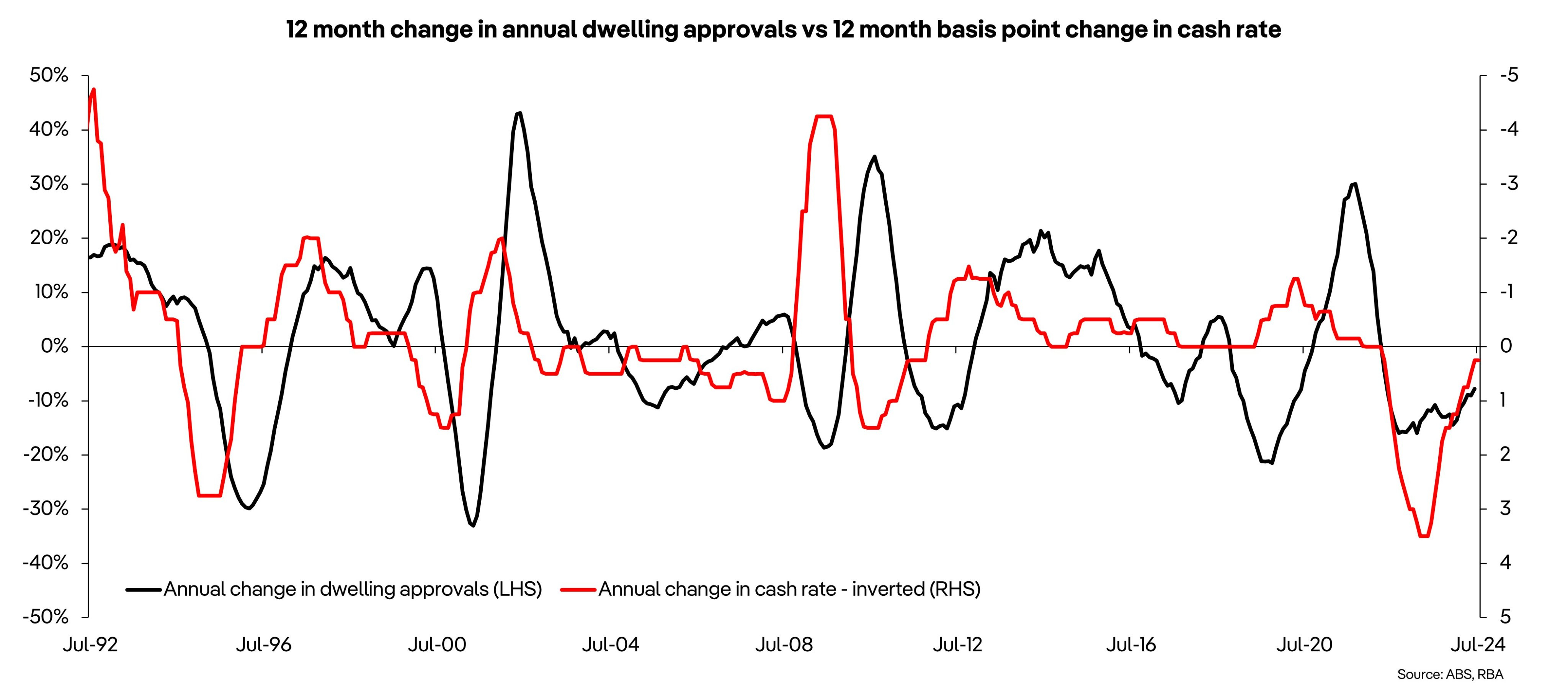
This fits with the cycle of housing construction in Australia. REA Group’s Cameron Kusher shared this chart recently, showing declining interest rates leading housing construction cycles (though of course demand growth and interest rates are themselves not independent).

Other rates of housing production mean that abnormal returns can be had by making certain asset swaps shown in the above diagram. This is the only condition where the gains from waiting equal the gains from producing homes, and the rate of return is equalised across all asset trading margins.

But this is very much the edge of knowledge as I said.

In fact, an academic paper of mine where I first looked at the question of equilibrium rates of housing production found the opposite relationship with interest rates (more on that paper here). In this setup, where a single landowner optimises their net profit flow, higher interest rates mean a higher cost to waiting (i.e. by holding land instead of cash) and hence a faster optimal rate of supply.

How these individual-level and market-level incentives interact, regarding the return to holding other assets (the interest rate), is an unresolved issue at the cutting edge of economic thinking on housing supply. Either (or both) of these approaches may be wrong. Or both incentives may exist, but interact in ways we don’t know about.⁵

In sum

Knowing that markets trade-off production across time, and specific intertemporal conditions required to make housing production worthwhile today, are just the first steps in understanding how taxes and regulations might affect the rate of housing production.

How do changes to taxes, monetary policy changes, and regulations on development affect these outcomes? We honestly don’t know.

The thing is, this type of dynamic optimisation must happen in every market. Toyota’s production of Prados will be responsive to demand growth and they may also reprice higher if demand grows quickly, and lower prices if demand is falling.

Despite the widespread confidence in our knowledge of housing supply, there is a theoretical black hole here. This post has taken you to the event horizon of knowledge.

But I hope by coming this far, you are ahead of 99% of pundits who yell “supply and demand, stupid” to anyone who wants to understand markets better.

1. I am confident that most people don’t understand what supply and demand curves represent. They’ve internalised the language of economics they have been taught, which has been reinforced by others using it (social validation). But supply and demand is just a shorthand way to explain the bigger concept of equilibrium. The problem is that equilibrium happens across many dimensions, and supply and demand is a way to represent many different trade-offs. It is the assumption about what equilibrium condition should hold that determines what supply and demand mean for any trade-off. For example, this explanation from Brian Albrecht is quite good at showing that supply is just a representation of opportunity cost in the dimension of interest.

2. Here’s a copy of that final version.

Murphy Dynamicmodelhousing 2018

1.31MB ∙ PDF file

Download

Download

3. The funny thing is, it is possible to draw a supply and demand diagram for each of the markets noted by the arrows. Supply and demand diagrams are merely a way to visualise the general concept of a trading equilibrium and how prices change when people change their willingness to buy or sell goods or assets.

4. I’ve previously called this sensitivity market thinness, which if you imagine the bid and offer curves on an asset trading exchange represents the inverse of the slope of the offer curve.

5. Another issue at the edge of knowledge is the tension between the price levels versus rates of price change effect on the choice to delay or accelerate homebuilding. For example, if you think that prices will be higher in the future, real options logic suggests you don’t build now, but build a bigger and more profitable housing project in that future period when prices are expected to be higher. But if the rate of price growth is high, then you want to accelerate the rate of production of housing per period now. Yet, the only way for future prices to be at a higher level in the future is via the rate of price growth. However, the rate effect is to accelerate housing production and the level effect is to slow or delay it. I will write more about this in the future.