
The FIVE ECONOMIC FORCES of housing markets
And why we need to understand how property markets operate to make informed policy changes


A bonus post today that has also been published at Aziz Sunderji’s terrific Home Economics substack. I had a great conversation with Aziz earlier this year on the FET podcast.

As always, please like, share, comment and subscribe.
In The Great Housing Hijack I outline the five equilibrium forces that determine property 1) prices, 2) rents, 3) their spatial variation, 5) density, and 5) the rate of new production.
These matter.
Too many contributors to the academic and public debate on housing have little economic notion of where prices come from, or why property markets deliver certain outcomes.
Grab your copy of the book here.

What’s an equilibrium?
To get started in understanding these forces we need to understand the logic of trade and equilibrium pressures.
Consider the below image of two supermarket checkout queues.

Because people can swap (trade) queues this situation is not an equilibrium. There is an arbitrage opportunity for the people at the back of the long queue to swap and get checked out more quickly.
The below shows these trades and the resulting equilibrium checkout queue length.

Will checkout lengths always be exactly equal? No. But they cannot stay far from this equilibrium point for long and the force of trading choice keeps the lengths tied to this outcome.
Equilibrium is a fundamental idea in economics. But it is often applied haphazardly.
My approach to housing markets refines our understanding of equilibrium forces driven by trading choices that constrain property market outcomes and looks at these forces across the many economic dimensions involved in property markets and housing.
Where do home prices come from?
Most people would say supply and demand. That’s a start. But it doesn’t tell us much more than that sellers and buyers agreed to prices.
I mean, who else sets the price?
Supply and demand is merely a description of market price adjustment. It doesn’t tell us why buyers were willing to pay a certain price, nor why sellers want to sell and are willing to accept that price. It doesn’t tell us anything about the broader equilibrium trading forces in the market.
The trick to understanding property asset market prices (yes, housing is an asset) is that every dollar spent on a home can be spent on any other asset in the economy. Homes can’t be priced for long at a level whereby the return on a dollar invested in housing is far out of whack with the rates of return on a dollar invested elsewhere.
The rate of return from rents and capital gains on housing must track closely the prevailing rates of return in other asset markets over the long term.
This is why monetary policy, whereby the interest rate on bank deposits is lowered or increased, has a substantial effect on home buying and prices.
Lower returns on cash assets make the returns on housing at the prevailing price seem more attractive. To use the checkout analogy, money leaves the cash queue and goes to the housing queue. Vice-versa when interest rates rise (though there are longer lags and more price stickiness when it comes to declining asset prices).
An easy way to think about this equilibrium relationship with other assets is that homebuyers can either rent a home from a landlord or rent money to become their own landlord.
Where do rents come from?
If housing asset prices come from equilibrium forces that ensure rates of return can’t diverge much from other asset markets, where do rents come from that determine that return on housing?
Rental equilibrium forces come from the trade-off between spending an extra dollar of household income on rent or an extra dollar on other goods and services.
Many people think that this means that with enough extra housing, rents will fall as a share of income across the market.
This is wrong.
Yes, spending a smaller share of income over time does happen for many goods, like food and clothing, where demand is easily saturated.
But not housing.
As incomes rise, households tend to do one or more of the following.
Move to a bigger home
Reduce the number of people per household
Renovate or improve homes
Move to a better location
Because a better location is a relative concept, there is a type of tournament economy for the best-ranked locations. Across the market, people compete in that tournament to climb the ranks of relatively superior locations until they spend roughly a fixed share of their income on housing rent.
Surprisingly, because of these adjustments in household composition and location, the actual quantity of dwellings and people is not so important for determining this rental equilibrium. A few decades ago there were 3 people per dwelling on average in small homes, and now when there are 2.5 people on average in large homes, and this equilibrium seems to hold.
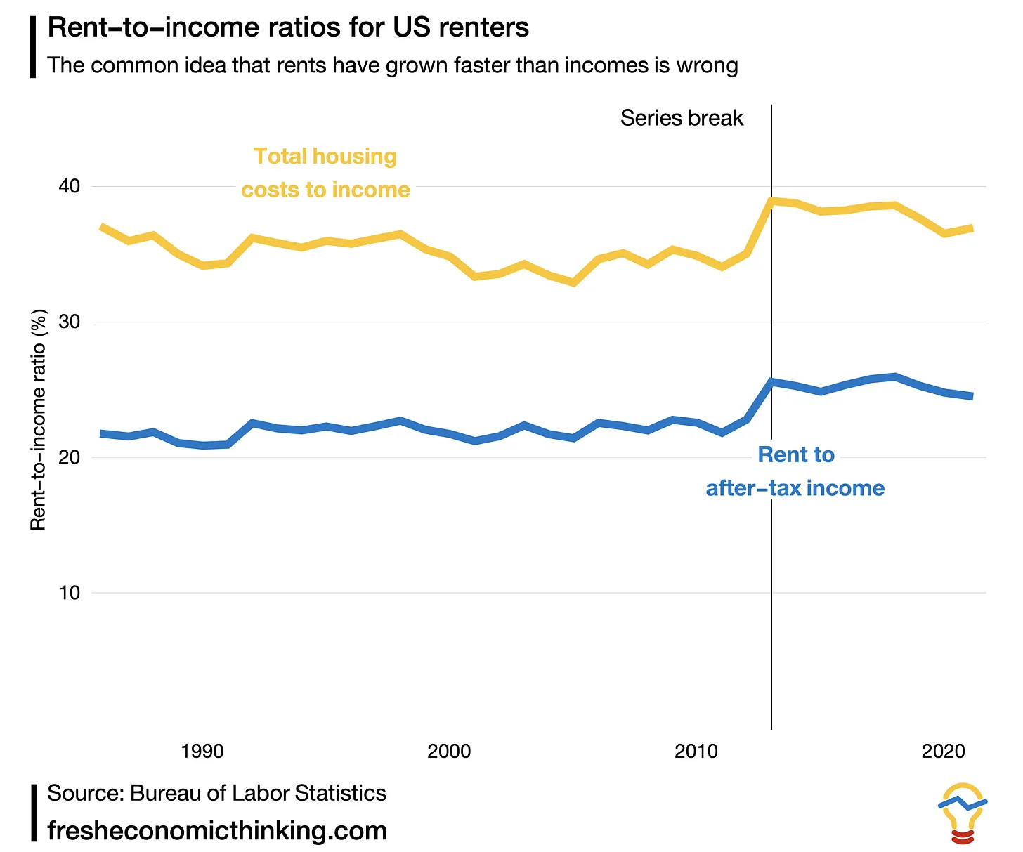
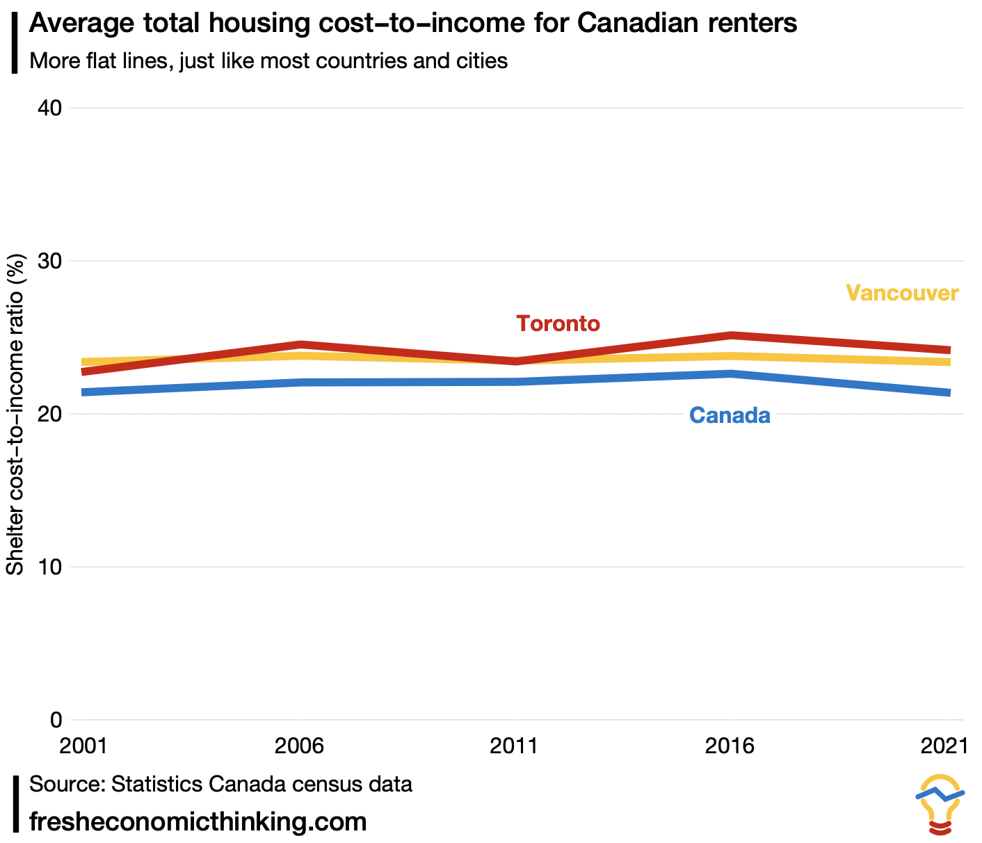
And we do see that in the United States, Canada, Australia, and New Zealand, rent-to-income ratios have been flat for many decades, as expected. In fact, in Australia’s first inquiry into rising rents in Sydney back in 1911 rents were then 20% of income, the same as 110 years later in 2021.
Here are some charts.
The only way to get rents to fall below this equilibrium is to limit the ability of renters to try and move to better locations (to trade or swap queues). This is the same way we can make the supermarket checkout queue shorter—stop people from the long queue trying to trade into the short one.
Another insight from the rental equilibrium is that inflation in non-housing goods means that renter households can pay more for rent because that means giving up fewer other goods and services for an extra quantity or quality of housing. This is the opposite of what many people might expect. Some might think that if goods and services have risen in price then households have less left over for rent, so rents should fall when there is inflation. This is wrong.
Spatial equilibrium
Why are rents higher in some places and not in others?
The answer is that there is an equilibrium in another dimension—across space (or location). People can move to different locations and will do so if the value of that move exceeds the extra cost of housing at that location.
The ability to swap queues—from one location to another—means that the difference in rents between locations reflects the total quality of life difference between locations.
The example below is from my book The Great Housing Hijack.
Here, the Jones family values living in House A at a prime location at $600 and the identical House B at an inferior location at $350 based on their own household’s preferences, work and family needs. The Lee family values House A at $700 and House B at $350.
If the Lees lived in House B and the Joneses in House A, they could swap homes and both be better off. Alternatively, if both homes were owned by another landlord, the Lees would end up renting House A at $700 and the Joneses House B at $400.
The $300 difference in rent for the identical home at a different location is the market assessment of the relative value of each location.

This is why I think many renters argue against gentrification. They think these local investments will make their location relatively more desirable to others and that they will then have to pay higher rents to compete with others just to stay put.
What determines housing density?
There are many debates about how densely we should develop cities. But too often economic analysis is missing.
Density is another dimension where equilibrium forces exist in property markets. Before a project is built, there are multiple queues—less dense or more dense. The queue that maximises the net value to the property owner is the one that is the equilibrium density.
This equilibrium force affects physical housing outcomes only at the time a new housing project is being irreversibly committed to. All previous times do have an optimal density, but that doesn’t mean that housing at that density will be built.
The basic logic arises because there are diseconomies in constructing higher-density projects. To build a home worth the same value at a higher density requires more capital.
This is easy to visualise with high-rise apartments. The tallest ones happen only in high-value areas because the extra high value of an extra apartment can cover the extra cost of going higher.
But the principle applies just as well to detached housing subdivisions, townhouses and low-rise blocks.
You keep testing whether more density leaves you more value left over after necessary capital investments until you maximise that residual.

It is important to note here that every home has the “wrong” density as soon as it is completed. Markets change and so does the density that maximises value to the property owner.
It is also true that many different density projects can be feasible at a particular time (i.e. the net value of a housing project after capital costs exceeds the value of the current use of the property). Out of all the feasible projects, the one with the highest residual value is the highest value use.
How quickly should new homes be built?
It is common to think that all feasible homes are immediately built and this is why we need to change the planning system to create more feasible housing development locations.
That is wrong.
Generally, there is an enormous pool of feasible housing projects either approved or allowable in the planning system.
For example, in Queensland where I live, there are likely many millions of apartments that are feasible and allowable. Currently, there are 125,000 apartments with planning approval. But only about 6,000 apartments are built per year.
The rate of housing production out of the pool of feasible projects is regulated by a market equilibrium as well—the absorption rate equilibrium.
To pick up the supermarket checkout analogy again, the two queues are 1) build today or 2) build in the future. The rate at which projects shift queues is the rate at which new homes are developed.
When new home buying slows down, rather than decrease prices to keep selling and building new homes at the same rate, property owners also slow sales and delay more homes.
And in a boom, they bring forward projects to meet rising homebuying.
Making projects feasible does not mean they will be built today. They might be more feasible tomorrow!
I highly recommend this detailed article on the topic of optimal delay in housing production.

So what?
Housing debates often ignore these fundamental economic equilibrium forces.
Many people think we can make rents fall in a single city by creating more feasible new housing projects there, ignoring the rental, spatial, and absorption rate equilibria.
The diagram below shows how density and the rate of new housing production (the absorption rate) are distinct concepts, but too often confused.
We can build four new homes per year at low or high density, or build eight new homes per year at low or high density.
Most people assume that creating more high-density feasible projects means that not only will density increase, but the rate of housing production (the absorption rate) will too. For some reason, they slip a hidden assumption into the word supply that a fixed number of projects must happen each year, and the more homes in each project, the faster we get more homes.

If we want to change housing policy, the least we should do is first understand how property markets work and what outcomes are possible.
 | A guest post by
|
Here's an example of the absorption rate equilibrium. https://www.austinmonitor.com/stories/2024/02/austin-apartments-boomed-and-rents-went-down-now-some-builders-are-dismantling-the-cranes/
Notice the chart in the middle of the article entitled: "New apartments in the Austin area vs. average monthly rents, 2000 - 2023"
It's literally a classic exposition of how markets work. As rents fall, production quickly falls, and when rents begin rising again, production picks up. And notice, in the long term, rents have more than doubled despite increased units. A great example of how markets won't overbuild for long, and won't build rents down in the long run. They will follow rents.
In this particularly case, Austin is well known to be a highly elastic US building market. It's the YIMBY deregulatory mecca. Yet elastic building has not produced lower rents. The Austin market, like the California market, is driven by rapid increases in high-wage job densities.
I would be willing to bet that there is directly relationship between the long-term average slope of rent increase shown in the chart and the long-term increase in median income over the same time, normalized for increases in construction costs. Expensive new luxury apartments are built to accommodate influx of high wage employees, and stop being built when that in-migration stalls or ends, or must wait for area-wide wages to increase.
Here's an example of where housing construction is being stalled because interest rates offer a better investment. It shows construction costs set a floor for rents, and it shows that new production won't take place until there is enough market support of high-salaried job growth to create new markets of potential renters who can afford the rents high enough to produce competitive yields to investors.
https://www.smdailyjournal.com/news/local/most-of-san-mateo-s-large-developments-on-hold-by-finances/article_45d447e4-0b86-11ef-8256-af01ceecaed0.html?utm_medium=social&utm_source=email&utm_campaign=user-share
"Most of San Mateo’s large developments on hold by finances"
In case you hit a pay wall, here are the money quotes:
"Mike Field, principal at Mecah Ventures, said high interest rates and escalating construction costs remain some of the primary culprits of construction hold-ups, but it’s also a consequence of ongoing remote work patterns and therefore, declining or plateaued rents.
“Lenders are looking at deals, seeing that interest rates keep going up, rents are not going up, and they’re saying the deal is going to be underwater when it gets built,” Field said, adding it suppresses developers’ appetite as well. “The demand issue for multi-family [residential] and the lack of rent increases is driven by the back-to-office delay. They’re intrinsically tied together.”
...
“Equity investors are looking at the anemic returns on multi-family development deals, and saying, ‘Why would I go invest at 4.5% or 5%, when I can go buy a 10-year treasury bond at 5.5% and take no risk?” Field said.