
We DON'T KNOW if housing construction productivity is RISING or FALLING (Part I)
What we got from Australia's Productivity Commission recently were silly methods without sound economic logic


PART II IS NOW AVAILABLE HERE!
Since we know little about the causes of productivity increase, the indicated importance of this element may be taken to be some sort of measure of our ignorance about the causes of economic growth…
- Moses Abramovitz, 1956
Last month, the Australian Productivity Commission (PC) released a report that began
Improving productivity can help fix housing affordability
Australian housing is increasingly unaffordable. Decades of inadequate supply coupled with high demand has driven this outcome.
In response, Australian governments have committed to build 1.2 million homes over 5 years – 240,000 homes each year. In the 12 months to June 2024, just 176,000 homes were built.
Governments have focused on alleviating constraints to new supply via changes to planning regimes. These are important reforms. But the speed and cost of new building is also a constraint on new housing supply.
Increasing the productivity of the construction process would lower construction costs – meaning more approved projects would be viable, increasing housing supply – even with no change in the size of the workforce, interest rates or the cost of materials.
But dwelling construction productivity has been stagnant at least for 30 years.
Fixing productivity will require a genuine focus on prioritising housing supply and affordability. This report provides policy directions for improving housing construction productivity by reducing the regulatory burden, streamlining and speeding up approval processes, supporting innovation and improving workforce flexibility to help turn the dial on this persistent policy challenge.
Download a copy here.

After you’ve read that, please take a look at a previous article of mine on the subject.

As I said in that article:
The puzzle for many is that labour productivity in manufacturing and many other sectors keeps increasing—we get more cars per car factory worker, more bottles of soft drink per Coca-Cola worker, and more agricultural produce per farm worker—but in construction, we get the same output value per on-site construction worker.
Why?
I want to focus on two things in this article—1) measurement issues and 2) the economics that helps us interpret those measurements.
That article was a deep dive.
This one dives even deeper. You’ve been warned!
I’ve broken it into two parts—Part I now and Part II in a few weeks time. I hope to explain to someone who isn’t an expert but is willing to follow the details of the logic why the analysis in the PC report doesn’t lead to the conclusions it makes.
There is a lot to get through to bring an intelligent reader who is not familiar with the issues along for the ride.
Background
Declining labour productivity in housing construction is a widespread economic concern in many nations. In February 2025, Australia’s Productivity Commission (PC) released the latest in a line of reports making a sequence of claims that:
construction labour productivity is declining,
causing higher construction costs, which in turn
increase the market price of housing.
There is no doubt that improvements in labour productivity across the economy improve living standards. It is also desirable for our regulatory environment to allow for, even encourage, new production methods and capital investment to facilitate this.
For example, the PC notes, as many have done before, that prefabrication in housing construction is a possible avenue for improving labour productivity.
Unfortunately, the sequence of three claims made is not supported by the data. We don’t know if housing construction labour productivity is increasing. Nor do we know if it is decreasing. Moreover, the link between productivity and house prices isn’t clear cut.
Concerns about the inability of construction productivity to keep pace with the overall economy are at least half a century old—as old, in fact, as the economic statistics used to measure industry-level productivity.
For example, Allen sought to understand in 1985 “[w]hy construction productivity is declining”. Further back in 1967, we learn from Cassimatis that “[a] persistent view in the economic literature is that productivity growth in construction is far below the national average.”
These days, you can find many attempts to measure and muse over the common pattern of construction productivity decline that is observed globally, either in the academic literature or economic magazines and websites.
The common cry is: “What is wrong with construction?”
But the economist, who realises that this sector is subject to market forces and pressures to innovate and economise as much as any sector, might want to be more circumspect.
Perhaps a better starting place is to ask: “What are we measuring and what would we expect that measure to show based on economic logic?”
That is the purpose of this article.
Rather than jumping to conclusions about the causes of changes in construction productivity, it is worth first reflecting on the puzzle of declining measured productivity during a period of sustained productivity gains across the economy. Is there some economic logic being missed that could explain the common trend across countries – one that each country, looking at its own experience, takes to be the result of local factors?
This “explainer” walks through the economic logic and measurement issues at the heart of the construction productivity debate and the recent PC report on the topic.
PART I - Labour productivity and its economic and measurement issues
What is labour productivity?
Productivity is the general name for a ratio of a given economic output to a certain input of interest.
Labour productivity is a class of productivity ratios where some form of labour input is used, whether in the form of work hours, total workers, or some other measurement.
It is an intuitive macroeconomic concept—with a given population and workforce input, an economy with higher productivity is an economy that can produce more valued outputs (numerator) for each person (denominator).
The way that labour productivity ratio’s outputs and inputs are measured is quite important.
Labour inputs can be work hours, the number of jobs, or some quality-adjusted metric that captures the various skills in the workforce. Which labour to include is not clear. Is it only on-site labour? What about upstream materials manufacturers? And what about the labour used upstream to build manufacturing facilities?
How much labour is used to make a product is not an easy question. This is why similar questions, like how much energy is used to make a product, are hard to grapple with for concerned environmentalists. The same economic and statistical limits mean we don’t ever really know the answer to either question.
Housing construction outputs are also tricky to measure.
Often, the number of dwellings is used (as the PC did in part of their analysis). But the quality and size of dwellings vary a great deal over time and space. It must require more people to make bigger and better houses. To deal with this, quality adjustments can be made to estimate a real measure of housing (adjusting for quality change, just like real prices adjust for inflation).
Another way to measure housing construction output is by using the total value of housing construction contracts. This overcomes some, but not all, quality adjustment issues. A problem here is that about 80% of the cost of construction comes from off-site inputs like materials. Why include only the labour involved with the final step in production, which accounts for only 20% of the total cost, but include in the output measure all the inputs like materials and contracted services, which make up 80% of the cost? It is like including only the labour at the car dealership, the last stage of production, but ignoring the labour at the car manufacturer when looking at the labour input needed to create the total car value.
To overcome this issue, it is possible to measure only the Gross Value Added (GVA) in the housing construction sector, not the total construction cost. GVA is the construction contract price minus non-labour inputs. This is the output measure the PC uses in their main analysis.
In the end, most labour productivity measures are ad hoc and often not comparable. Even classifying businesses into specific industries to know what industry is being measured is tough to do. Yes, there are groups of specialist economists working on all these measurement issues. But they’ve never found a practical way to measure the concept they have in their mind.
What the Productivity Commission did
Australia’s Productivity Commission (PC) looked at the labour productivity in the residential construction sector and concluded that their “new estimates of housing construction productivity tell a story of decades of poor performance.”
They claim that improved labour productivity in housing construction “can help fix housing affordability” and direct their policy recommendations towards “alleviating constraints to new supply via changes to planning regimes” and reducing “regulatory impediments” that get in the way of “prefabricated and modular construction.”
The mechanism by which this is thought to occur is that “increasing the productivity of the construction process would lower construction costs – meaning more approved projects would be viable, increasing housing supply – even with no change in the size of the workforce, interest rates or the cost of materials.”
They explain that in the past three decades that
• the number of dwellings completed per hour worked by housing construction workers has declined by 53% (physical productivity)
• gross value added per hour worked – a more comprehensive measure that controls for quality improvements and increases in the size of housing – has declined by 12% (labour productivity)
Like many previous authors from Australia and around the world, they have jumped to the conclusion that what they have measured is what they understand the concept of productivity to be.
What did the PC measure?
First, they counted the number of new dwellings produced as the output (the numerator) and the number of on-site work hours as the input (denominator) and called this Dwelling construction physical productivity.
We know that changes to the quality and size of dwellings make this metric economically rather meaningless. For example, it is possible to increase this measurement of labour productivity by building much smaller dwellings than desired by homebuyers. Because of this serious and well-known issue, I ignore this metric in the following critique.
Second, they added up the Gross Value Added (GVA) of residential builders and on-site contractors (which are part of an industry called Construction Services) as the output (the numerator) and the number of on-site work hours as the input (denominator) and called this Dwelling construction labour productivity.
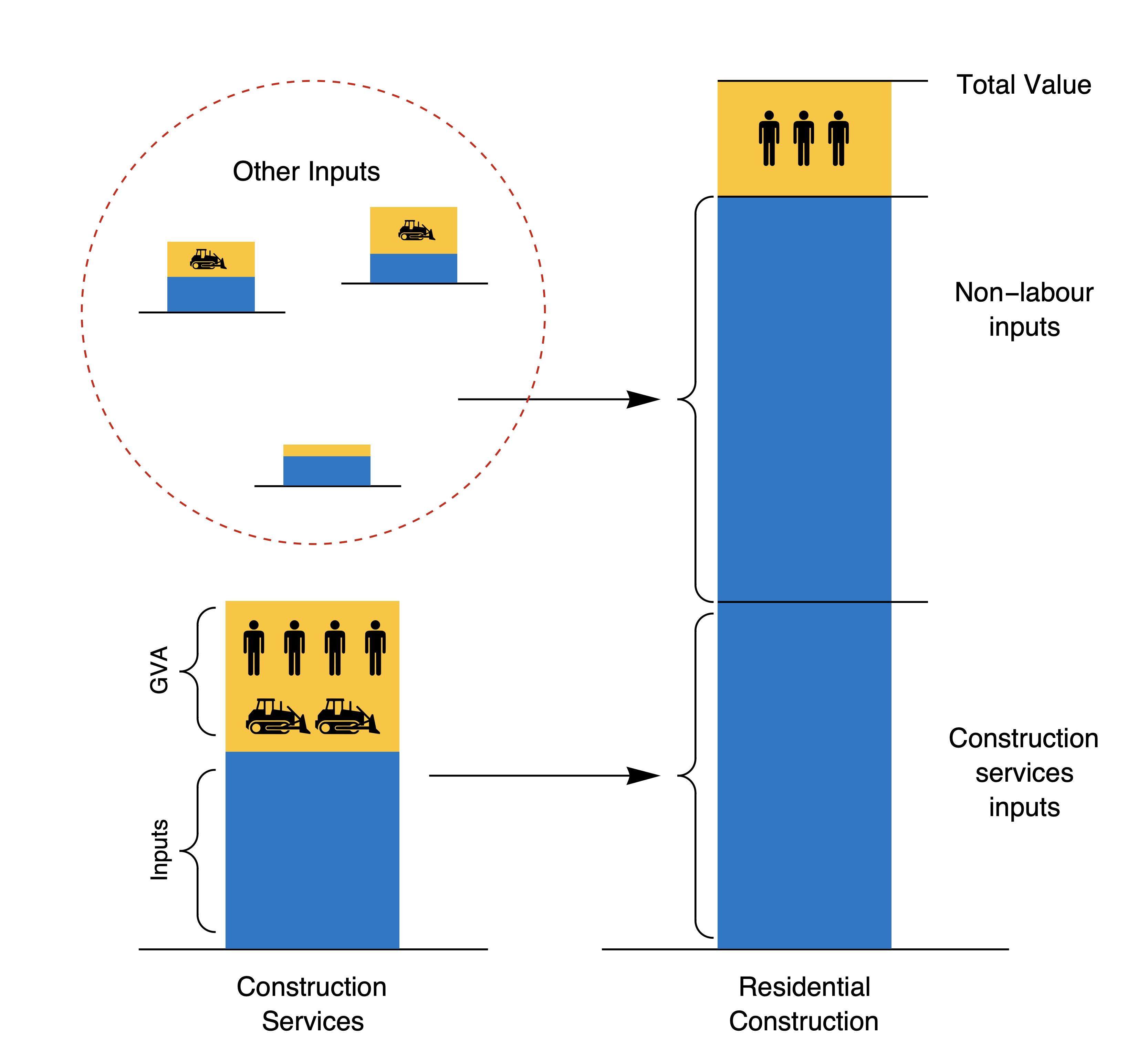
The diagram below helps to explain how this is done (it is a good one, helps to show the main point, and is worth the paid subscription to drop the paywall).
The right column shows the total value of a construction contract for a residential builder. The blue section of the costs are all the non-labour input costs from on-site contractors (bottom) and materials suppliers (middle). The yellow section (top) is the cost of wages to residential building company workers plus the profit margin for the builder. This section—the profits and wages— is the GVA of the building company. It is how much value they added to the production process.
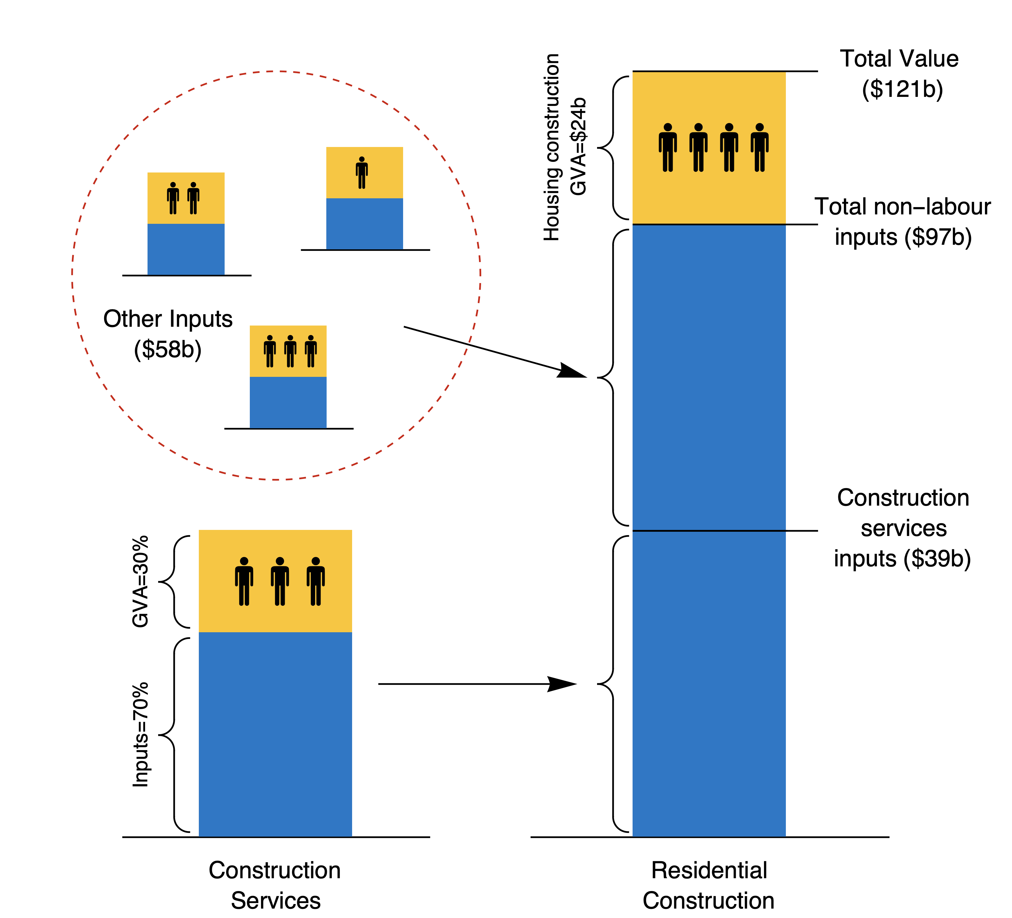
To provide some sense of scale to how this looks across the whole industry in FY2022-23, Residential Construction as a category of production had about $121 billion of output (learn more about the industry categories here). It used $97 billion of inputs (blue) and had a Gross Value Add (GVA) of about $24 billion (yellow).
The left column (and the floating columns) shows the rest of the picture. Most on-site construction workers are independent specialist firms, like plumbers, electricians, bricklayers, roofers, and so forth.1 These businesses are classed as Construction Services and typically involve on-site work. They are about $39 billion of the $97 billion of inputs (i.e. about 40% of total non-labour and non-profit input costs).
It is important to note that Construction Services are not professional services inputs such as from engineers and architects, nor town planners. These services are generally considered to be part of a completely separate output and are classified as Professional, Scientific and Technical Services. These services are paid for by property owners in parallel to construction services.
The Other Inputs includes materials, and as the PC itself notes, things like the “offsite production of prefabricated buildings and building components” which is the output of the Manufacturing industry, and the cost of “infrastructure and utilities” which are the output of the Heavy and Civil Engineering Construction Sector.
Of the total Construction Services inputs into new housing, about 30% of their total cost is GVA, meaning that 70% of the value of their output comes from upstream inputs to these services.2
To summarise, of the total $121 billion cost of housing construction in 2023, the GVA considered in the PC analysis of Dwelling construction labour productivity includes $24 billion from the Residential Construction industry category (the yellow in the right bar), and 30% of the $39 billion of Construction Services inputs (the yellow on the left bar), or just $37 billion in total—this equates to only 30% of the total construction cost of homes.
Everything else is left out of the output measure (the numerator).
All non-construction costs, such as professional consultants like town planners and engineers, are ignored, as are profit margins for developers (rather than builders) and many other parts of the new housing development process.
As well as being the value added by these contractors and builders, this GVA figure is, by definition, also the sum of the profit margin (return on capital) and wages for these firms. Any resulting labour productivity metric is also a profits and wages per on-site worker metric. This matters when it comes to an economic interpretation of the figures, which is explained in detail later.
The labour input measure used by the PC is the sum of hours worked in the Construction Services and Building Construction industries, scaled by the proportion of each of these sectors devoted to residential construction—a proportion that comes from other surveys to help triangulate a reasonable estimate of the labour associated with the GVA used in the analysis. It’s rough, but I think it works.
Using this second GVA metric of Dwelling construction labour productivity, the PC found the patterns shown in the chart below over the past two decades.
Relative to the GVA per hour worked over the whole economy (black dashed line, which is also by definition Gross Domestic Product (GDP) per hour worked) the value added in the residential construction sector per hour worked fell for detached houses (yellow line) or fell, then grew, then fell sharply again, for attached dwellings like apartments and townhouses (red line). The net productivity change for all dwelling types combined was a slight fall.

Does it pass the sniff test?
Before going further into the economics of why this metric of labour productivity might rise and fall and why declining relative labour productivity in construction has been a topic for half a century, it is worth pausing to undertake a sniff test on the PC’s results.
Do we trust that the pattern found represents the underlying concept of productivity that we hope to measure?
Consider the Dwelling construction labour productivity for attached dwellings (the red line). Do we believe that changes in production technologies, skills, and regulations, which are thought to be important determinants of productivity, were the cause of an 86% increase in productivity from 2008 to 2014, only for these same factors to cause a 30% decline in the five years after 2018?
To be more specific, are there reasons unrelated to production technologies, skills and regulations for why the measured productivity of attached housing construction varies so much over the property cycle?
The number of attached dwelling building approvals grew from around 45,000 per year in 2009 to around 115,000 per year in 2015—a 2.5x increase in the period when labour productivity apparently also grew 86%.
If there are good economic reasons for this variation, do they also explain the stagnation or decline in measured productivity for detached houses that is a long-term and global phenomenon?
After all, the PC itself looked at similar labour productivity measures from many nations and found that Australia’s performance was the best when compared with France, Germany, the United States, the United Kingdom and Sweden. The report could have gone with the title “Australia’s world leading housing construction productivity: What others can learn”. But choosing to downplay Australia’s outperformance and ignoring the obvious questions about the implausibly large swings in attached housing productivity suggests that little economic reasoning or critical scrutiny was applied.
Before drawing long-bow conclusions about town planning, building regulations, prefabrication, and more, understanding the measurement and the economics behind it seems an important first step.
What Baumol would expect on construction productivity
William Baumol and William G. Bowen, back in 1964, described the problem of productivity in the performing arts. Later debate and analysis labelled their observations Baumol’s Cost Disease, which explains the mechanisms by which incomes can rise in a particular area with no productivity gains due to productivity gains elsewhere in the economy.
His example was that "[t]he output per man-hour of the violinist playing a Schubert quartet in a standard concert hall is relatively fixed, and it is fairly difficult to reduce the number of actors necessary for a performance of Henry IV, Part II."
He asked how the incomes of musicians increased over time despite the lack of productivity gains.
There are a couple of forces at play.
One is that musicians flourish on the back of economies of scale elsewhere, such as in the distribution of music, with radio, records, cassettes, compact discs, and now streaming. Indeed, large concert halls are an attempt to scale up the output of performers to a bigger audience to increase the effective productivity of a performance.
Another force is that because workers can switch between jobs, they will want to go into the high-wage jobs in high-productivity areas. To keep workers in relatively low productivity service work, you must pay them enough to bid them away from those other high productivity parts of the economy. This is how productivity gains in one part of the economy lead to income gains across the whole labour market —the ability of workers to shift between jobs equalises pay for similar work regardless of the underlying economic productivity of each sector.
This second reason is why historical productivity gains in agriculture or manufacturing pushed up wages in other parts of the economy with no productivity gains.
So what?
Several predictions follow from Baumol’s economic logic. This helps to establish what we should expect to see when we look at productivity measurements.
Two main predictions are that:
The share of employment in sectors with high productivity growth falls, while employment in low productivity sectors rises.
Rising costs of the output of labour-intensive industries are not necessarily due to inefficiency, nor are falling costs due to efficiency. Sectors are interdependent.
The first is less important for our analysis of construction sector labour productivity. But it is worth dwelling on how the share of total employment for many decades has shifted away from agriculture, mining and manufacturing (where new technology has led to productivity gains) and towards service industries (where productivity gains have been minimal). Fewer people are needed for the same output—so despite rising agricultural, mining and manufacturing output, there are, on balance, fewer people working in these sectors. Despite this, it is the high productivity of these sectors that allows for higher real wages in all other sectors.
The second prediction is more subtle but more critical to understand to help interpret any attempt to measure labour productivity of a sub-sector of the economy.
Consider again the above example of the long-term shift of employment to cities due to productivity-enhancing activities in agricultural areas, increasing crop yields and minimising necessary labour, and so forth.
The result of this has been that measured labour productivity is higher in the cities with many service jobs compared to the regional and rural areas.
Why?
Because service jobs generally have high education requirements and fetch high incomes relative to rural work, a premium must be paid for these workers above what they can earn in agriculture. Since the value of any output must cover the cost of these high wages, measured labour productivity will be high.
Recall that the GVA of any sector is also equal to the sum of wages and profits.
This means that since corporate profits of high productivity mining and agricultural companies are recorded in the cities where headquarters are located, and high wage people work there, the sum of GVA—wages and profits—divided by the number of workers in the city is much higher than in the rural areas where actual new technology and productivity enhancement was made.
This is a hidden economic interdependency that must be understood when trying to interpret labour productivity measurement.
Let’s dig into this idea further by looking at a single company.
BHP, the Australian mining giant, has its global head office in Melbourne’s central business district. But the service jobs in that office only exist because of the productivity of the physical mining operations scattered around remotes areas of the nation.
If you removed the head office, the mines could still operate and be productive.3 But if you removed the mines themselves, the head office would be totally useless. It is the productivity of the mining that allows for more people to work in the service-based, low-productivity office.
What happens when we measure the productivity of BHP’s head office and compare it with its mines?
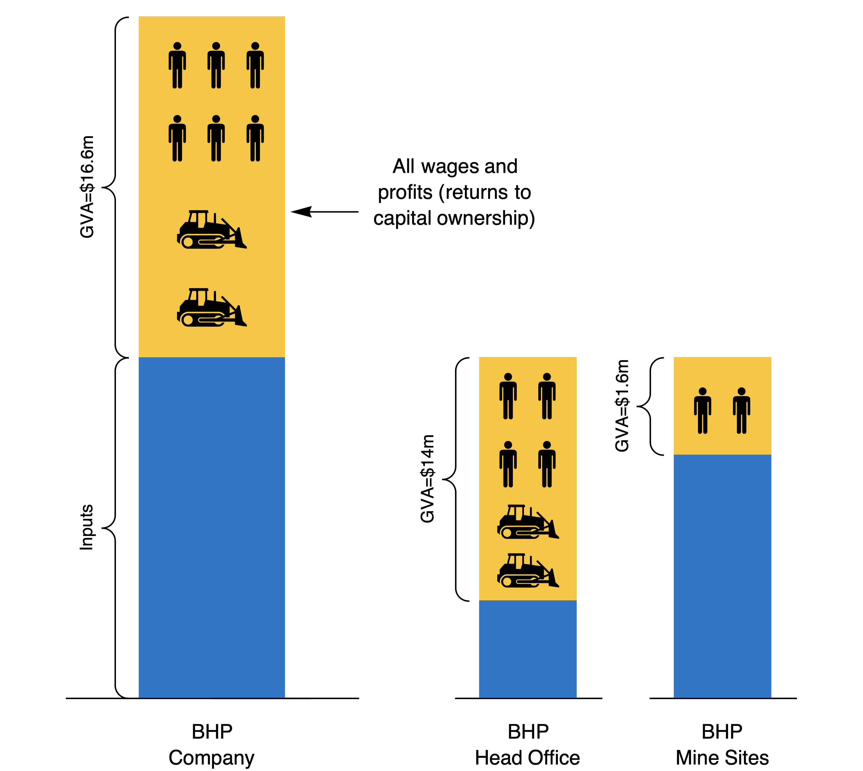
The below diagram shows what happens here. The total on the left includes all mine-site workers and the head office workers for the whole company (each stick figure represents 10 workers in our simplified example).
But what happens when we break down the sub-industries of mining and corporate services?
Now, all the corporate profits and high wages of the service staff and senior personnel are recorded at the head office. Divide that large head office GVA by the number of staff and we get a high labour productivity measurement. To put some numbers on it, if corporate profits are $10 million (from ownership of capital, represented by the bulldozer in the diagram) and 40 people at the head office earn $100,000 each in wages, then we have $14 million of GVA [$10m + (40 x $0.1m)]. Divide that by the 40 workers to get a labour productivity of $350,000 per worker at the head office.
What about the physically productive mining sites themselves, which is the construction sector of the BHP economy doing the on-site work?
Here, only the wages of local workers are in the GVA of this sub-industry of BHP. If the 20 on-site workers earn $80,000 each on average, then the labour productivity of this part of the business is just $80,000 of GVA per worker, or just 23% of the labour productivity of the head office part of the business.
In other words, when we break apart the BHP business, our productivity measurement says that the head office is more than four times more labour productive than the actual mines themselves that create the product the company sells and upon which the head office relies for its existence.
Would we interpret these figures to mean that mine-site workers are underperforming?
After all, the average labour productivity of BHP is $277,000 of GVA per worker ($16.6 million total wages and profits divided by 60 total workers) and the head office is 26% above the average, while mine site operations are 71% below this average.
Or would it be more sensible to realise that productivity measures often miss the interdependency of economic activity and that Baumol was right not to draw strong conclusions from measured productivity in subsectors of the economy?
The latter must be the case.
This lesson of interdependency between sectors, and hence where productivity gains end up in our measurements, is too often missing from our interpretations of productivity measurements, with the PC report being the latest example.
How productivity measurement misleads
Let’s take this economic background and use it to look at ways in which measured productivity in residential construction might rise or fall based on interdependencies with other sectors without being anything to do with regulations, technology or skills in that specific sector.
We are trying to learn how measurements will mislead without an economic understanding of the interdependence of labour productivity.
These examples not only apply to the GVA-based labour productivity metric used by the PC, but they apply to varying degrees to construction labour productivity estimates that use contract values or quality-adjusted dwelling output metrics as well.
The interdependence of economic sectors cannot be ignored.
Relative wages, on-site labour and builder profit margins
Remember that the GVA of an industry is both a measure of the value added and a measure of the sum of wages (or self-employed labour income) and profits in that sector.
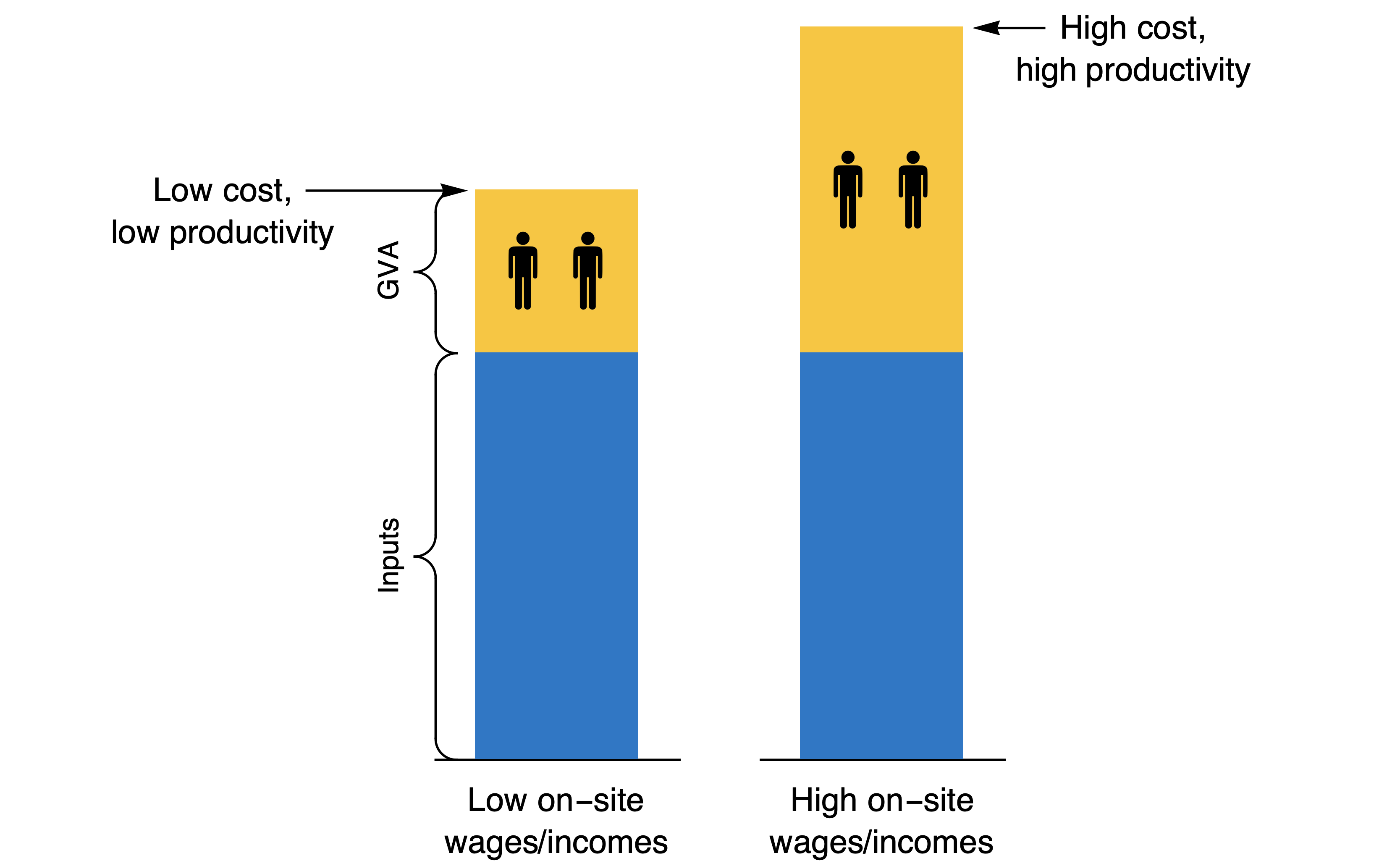
If wages rise for on-site workers in the residential construction sector, whether that is the trades that make up the Construction Services industry category or the builders themselves, then GVA must rise on a per worker basis, raising measured Dwelling construction labour productivity.
The below image shows this, whereby fixed non-labour inputs are combined with either low- or high-wage on-site workers.
Notice that in this scenario, higher labour productivity is associated with higher total costs of constructing a home. It is usually assumed that higher measured labour productivity means lower cost, but this is not necessarily the case.
Looking at this situation in reverse makes that clear. Take a scenario of high wages, then bargain down the price of a build by getting lower-wage workers, and you reduce costs while reducing labour productivity (because GVA is the sum of wages and profits, and we’ve reduced wages).
The same economic logic applies to builder profits.
If builders make higher margins, it increases GVA in the residential construction sector, just like higher wages. In fact, labour income and profits are often indistinguishable in the residential construction sector, as most builders are single-person businesses—profits are their labour income. The residential construction industry is dominated by such businesses— the average building business has fewer than two people (see page 4 of the PC report).
The same logic of wages and profits applies to Construction Services. Therefore, one reason that Dwelling construction labour productivity can fall relative to the economy-wide average is from falling relative wages and profits in these sectors (and it can rise due to rising profits and wages). One example would be a shift in composition towards more volume builders of detached homes, with slimmer margins, and hence lower measured productivity despite their lower prices.
One of the main assumptions behind the PC report is that “[i]ncreasing the productivity of the construction process would lower construction costs” (p2). Yet we have just shown that this is not necessarily true and the reverse could also be the case.
Composition of on-site and off-site activities
Construction companies (builders) generally organise the inputs of others rather than invest in their own capital and machines to repeat the same automated processes. This makes sense, as construction jobs are all different, at different locations, using often different materials and techniques.
This is why prefabrication has been so difficult to do, despite repeated attempts and many billions invested.
The words “pre-fabrication” or “modular” are mentioned 74 times in the PC report, and their Recommendation 4.6 suggests removing regulatory impediments to this type of construction. This is all fine and good.
But remember, anything prefabricated must be small enough to be transported to many different sites and moved on-site efficiently, then be adaptable enough to deal with measurement errors and changes in other parts of construction. Brian Potter is an excellent source of analysis on the difficulties and history of these systems (here are one, two, three and four articles by Brian as a starting point).
In practice, volume builders of detached homes do repeat the same designs and are very cost effective, even if that means they don’t have high measured productivity nor prefabricate large sections off-site.
Here, I will show how huge productivity gains can be made in the home-building process without entering the measured productivity figures. I will show how pre-fabrication may lead to lower, not higher, measured labour productivity in the residential construction sector.
The logic is this.
Innovations in new capital technology or economies of scale in the production of housing usually make sense in off-site manufacturing of materials and components rather than on-site final assembly. Any labour productivity gains happening in these construction inputs won’t be measured in the residential construction sector.
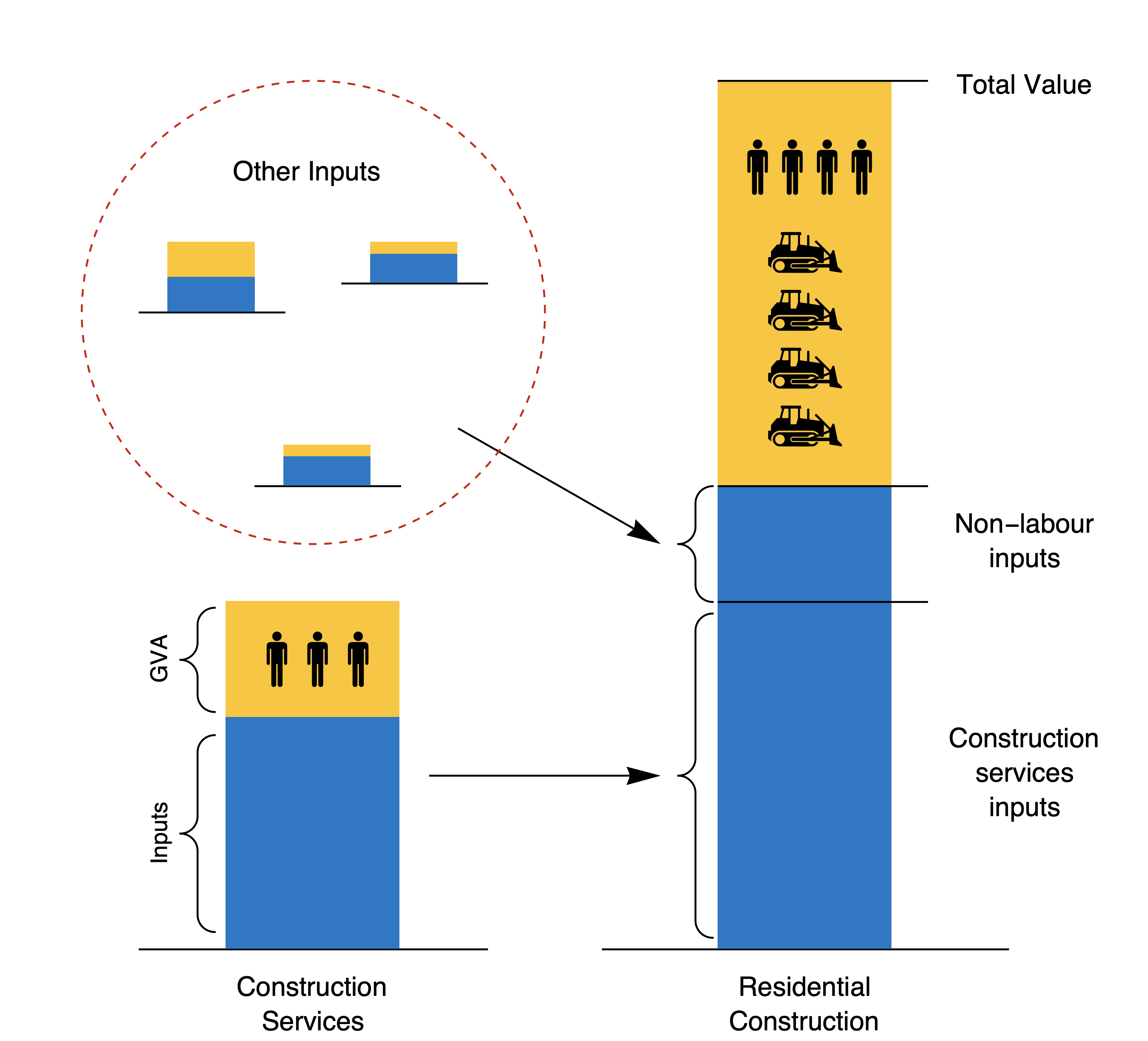
I will show using the below diagram how, if a highly productive new technique was implemented by a residential builder, sensible economic incentives would quickly remove it from measured labour productivity.
This diagram is a repeat of the general description of the inputs and GVA from construction services and residential construction sectors. However, this time, the builder (i.e. the Residential Construction industry) has new machines that boost the labour productivity of his projects (i.e. there is a lot of yellow GVA and not many people working on-site relative to that large GVA). These machines are represented by little bulldozers, but they could be any type of equipment. The important point is that the builder must charge an extra margin to cover the cost of this equipment—a margin that is in the measured GVA (the yellow part of the column) of his business alongside labour incomes.
The next economic question is: “Why would builders own a lot of capital equipment when they are mostly single-person businesses with a highly variable workload?”
Yes, higher margins are associated with large capital investments in machines and equipment, such as cranes, excavators and earthmoving equipment. But a builder won’t buy these machines, use them at one site, then park them until his next project is ready for them. The most efficient way to organise production is for capital-intensive businesses to specialise in offering these capital-intensive services on a project-by-project basis to residential and non-residential construction projects for many different builders, spreading risk.
The physical realities of housing construction are that the product is immobile, unlike vehicles, ships and indeed most transportable products, and that local conditions vary substantially (slopes, soils, standards for wind, rain, drainage, heating, etc). This is why high-productivity factory production is generally limited to small components that are not made by builders.
What does that look like in our diagram?
The machinery ownership that increases productivity gets shifted to suppliers, either Construction Services companies (whose GVA is in the PC measurement) or materials manufacturers (whose GVA is not measured). The GVA share of total revenue in Construction Services rises (it is 30% of output value compared to the residential construction category where GVA is only 20% of output value), and the GVA of the residential builders falls on a per worker basis.
Indeed, measured labour productivity on a GVA per worker basis in the PC report shows gains in the Construction Services sector, where they are expected, but not in the Residential Construction sector, exactly as described here, and just as Baumol’s economics predicts. The chart below illustrates.
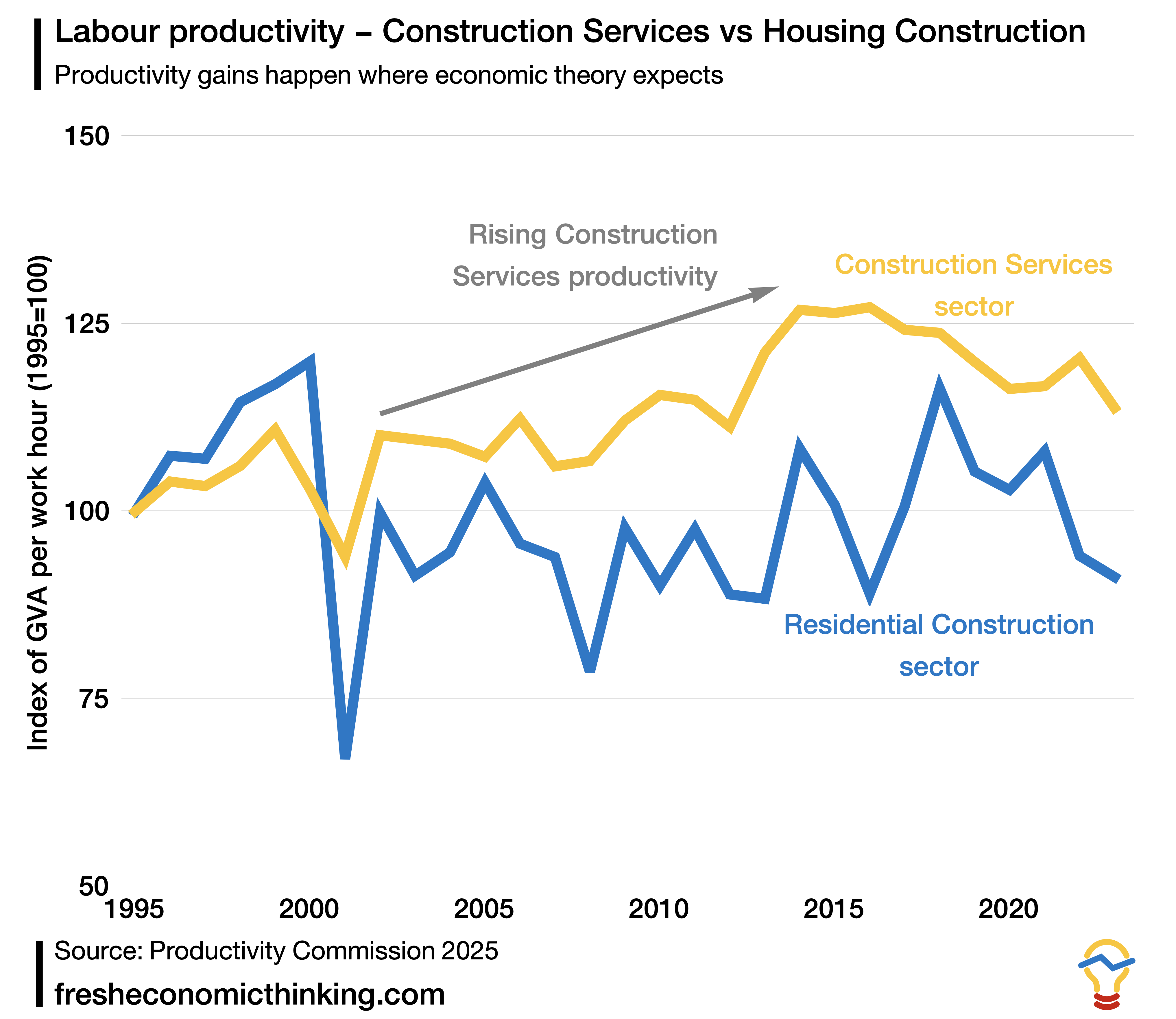
This compositional effect of productivity gains showing up in certain industries but not on-site building is probably the economic reason that higher measured productivity is observed in high-density housing. More on-site capital equipment owned by Construction Service companies, like cranes, excavation equipment, and so on, are used in these projects. More equipment-heavy construction techniques mean higher measured GVA due to the returns needed to cover the profits of owning that equipment, hence a higher measured labour productivity (GVA per worker).
One interesting dimension to this is that out of the total $121 billion of residential construction, only an estimated 60%, or $73 billion, was for renovations of existing homes in 2023-24. This is up from an estimated 34% in 2018-19. This is a big compositional shift, coupled with fewer apartments, that would cause a decline in measured productivity without there being any change in actual productivity.
To reiterate, the economic logic that returns on productive capital equipment accrue to their owners, not the users (the builders), is just like in the case of our BHP head office example. The returns from owning capital (corporate profits) were booked at the head office, not the mining sites where they were used. In residential construction, the returns on capital are booked to the owners of these inputs who lease them and provide services to builders, not to the builders themselves.
If prefabrication or modular construction was done by specialist firms who own the prefabrication facilities, rather than builders who manage the on-site assembly of components produced by these prefabrication firms, then measured productivity of builders may fall, not rise. This would happen in a scenario where high-wage skilled on-site labour could be replaced with lower-cost labour and if builder margins were reduced because of lower construction risks.
Prefabrication of homes is not part of the Residential Construction category of activities, nor Construction Services, but is part of the Manufacturing sector (ABS, 2025c). So shifting inputs to that sector would remove any productivity gains from the measurement of GVA per hour worked in the Construction Services and Residential Construction sectors. This shows a big gap between the analysis of productivity in the PC report, whereby measured labour productivity would not increase due to prefabrication, and the recommendations of the report that focus on prefabrication as a tool to increase productivity.
This compositional effect is like looking to musicians playing songs for productivity gains in the music industry. The productivity gains happen via the large theatres and the recording and distribution. If we ignore those gains and only look at the four musicians recording their string quartet, we will never find where the productivity gains are happening in the music industry.
So what?
Like many other analysts before them, the Productivity Commission has claimed three things:
construction labour productivity is declining,
causing higher construction costs, which in turn
increase the market price of housing.
I have explained why the first two claims are wrong, or at least, the analysis undertaken cannot support or reject these claims.
Firstly, the sniff test should have immediately led to caution.
Australia’s residential construction sector also saw the least decline in measured relative labour productivity of the peer comparison nations. Not only that, but measured productivity in high-density housing showed enormous and implausible variations that could not possibly be caused by the reasons suggested, such as regulation, planning and lack of prefabrication.
Indeed, it is foolish to put any weight on labour productivity measured by on-site labour use per new home when the type and quality of homes vary dramatically. But this measure was emphasised and shared by the PC despite being known to be misleading.
Second, I showed how Baumol’s economic logic shows the folly of measuring the productivity of one sub-part of production and making claims about causes of that change being from that sector, as there are strong economic interdependencies at play. The BHP example made clear how breaking apart the complex web of economic production leads to misleading productivity measures.
Third, I showed how variation in measured labour productivity is caused by variation in wages and profits of residential construction and services businesses, and how there are strong economic incentives for productivity gains to occur in upstream sectors of production that are not counted when looking at labour productivity of housing construction. It is possible, even likely, that higher productivity in housing construction would be associated with higher total costs per dwelling rather than lower total costs.
I also noted that looking to musicians and how quickly a string quartet records a song will not help you understand the overall productivity of the music industry, as productivity gains are made elsewhere and the musicians utilise those as inputs.
In short, measuring labour productivity for economic sectors is always problematic. There is no right way to do it and no right way to interpret any measurement. What we know from economics is that relative prices tell pretty much the full productivity story anyway. If prices for the same item fall relative to other prices, especially incomes, then there are productivity gains somewhere in the production process, even if we can’t measure or identify where they are occurring.
In Part II, I will dig further into the final claim made by the PC about construction costs and the market price of housing, as well as some of their suggested remedies, which focus on planning approval processes, innovation, economies of scale, and skilled worker “shortages”.
As you might guess, I will show that these claims aren’t supported by the analysis done either, and they too must be informed by economic logic.
As always, please like, share, comment, and subscribe. Thanks for your support. Find Fresh Economic Thinking on YouTube, Spotify, and Apple Podcasts.
Construction services comprise five categories: 1) Land development and site preparation services: the construction of roads on a subcontract basis for land subdividers; demolition of buildings or other structures; earthmoving; earthmoving plant and equipment hiring with operator; excavation; explosives laying; ground de-watering; land clearing; levelling (construction sites); removal of overburden; trench digging, 2) Building structure services: concreting; bricklaying; roofing; structural steel erection services, 3) Building installation services: plumbing; electrical; air conditioning and heating; fire and security alarm installation; awning, blind, curtain or shutter installation; elevator, escalator or lift installation; insulation installation, 4) Building completion services: plastering and ceiling services; carpentry services; tiling and carpeting services; painting and decorating services; glazing services, 5) Other construction services: landscape construction services; hire of construction machinery with operator; other services.
The ABS Supply and Use Tables that provide this industry-level information show how the outputs of one sector are used as inputs to another sector all the way up the value chain. The PC report scales the output of the Construction Services sector to the proportion used in the downstream Residential Construction sector to account for this.
Note that within Construction Services is a category of industry called Land Development and Subdivision, which includes the labour income and profits of housing developers. Most large-scale housing developers hold undeveloped land in one company structure and sell it to the development company at a price that minimises the income from development and maximises the return to owning the undeveloped land asset in the holding company. I am awaiting clarification from the Australian Bureau of Statistics (ABS) about how these classifications are made.
Without any structured corporate decision making, and perhaps without any expansions and capital upgrades that require the coordination of the head office service personnel.