A housing absorption rate formula—first cut
Housing supply is one of the most misunderstood processes in economics. The reason for this is that the core standard theory of economics is a static one-period model of production with a fixed capital endowment. They confuse the optimal density of dwellings, given the fixed capital of one unit of land, with the optimal rate of supply of new dwellings per period of time.
To be clear, the decision to supply existing housing to the rental market at any point in time is short-run production decision given a fixed stock of homes. That is why most homes that exist are not vacant. The marginal cost of renting (compared to keeping vacant) for a dwelling owner is typically far below the marginal revenue.
Building new homes is instead a capital allocation decision. Land and cash assets must be given up to build new homes. These assets earn a return over time and can be used in future periods instead of the current period. Building too many homes today depresses prices and rents, thereby reducing the return to both existing homes and homes you can build in the future.
So how is the optimal rate of new housing determined?
It is clearly not determined by the optimal density, as static models assume. Take a look at the figure below showing a housing subdivision in a street. The static theory says that if you approve a subdivision of five housing lots, you increase the rate of supply per period by five dwellings. They all sell in period one.

In reality, these dwellings do not sell all in period one (i.e. all in one day). They are drip-fed to the market over time, with one possible series of sales shown in the figure below. When I looked at the land banks of Australia’s top eight listed housing developers, the average age of their housing subdivisions and apartment blocks since their first sale, was ten years. The oldest was 25 years! They were still selling housing subdivisions approved in the last millennium.

This slow rate is optimal because housing developers are rational. Selling faster reduces both the value of the rest of their subdivision and the growth rate of the prices they receive over time. They are giving up future returns if they flood the market today.
What do those future costs look like?
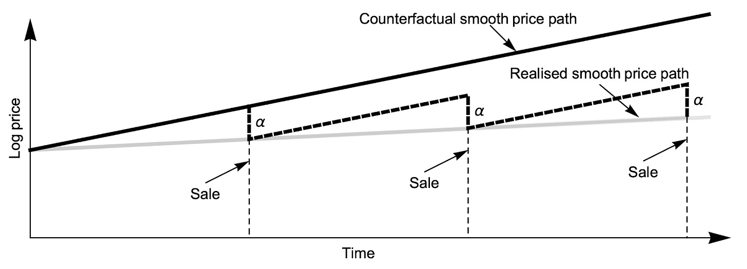
In the figure below we can see the effect of new dwellings sales on market prices and growth. The top line is the counterfactual price path if no new dwellings were supplied. Each additional dwelling when it is sold goes to the highest bidding buyer at that point in time, taking them out of the market and reducing the price to the second bid. This gap between the highest bid and next bid is labelled as alpha, and represents the “thickness” of the market in terms of how many people have bids clustered at the top of the curve. If you rank bidders from highest to lowest and get prices of 1.0, then 0.9, then 0.8, then alpha is -0.1 (the slope of this bid curve when buyers are ranked). If the market is “thicker” the bids might be 1.0, 0.95, 0.9, meaning alpha is -0.05.

Each sale at any point in time takes out a buyer and reduces the maximum price. Meanwhile, the other bids grow over time (or not) depending on macro and market factors. The next sale has the same effect, wiping off the next highest bidder and reducing the price, and so on.
So each sale has a pure price effect in terms of alpha. We can add these up on the above figure, and with a rate of sales of three per period, the price effect—the difference between the end of period price on the counterfactual end of period price is three times alpha.
This is standard economic theory, whereby increasing supply per period has a price effect. No surprise there.
But notice something else. The result of this pure price effect is that the price path is flattened compared to the counterfactual. Not only are end of period prices lower, but seen as a path, prices are growing more slowly.
The faster the rate of sales today, the lower future prices tomorrow. In essence, the pure price effect can be reinterpreted as a reduction in the growth rate of prices over time rather than a static price effect.
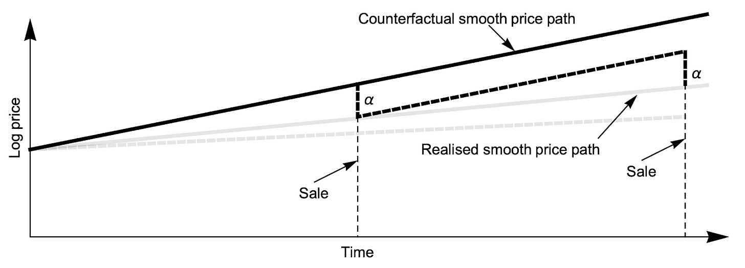
We can see this in the figure below where we reduce the rate of sales from three per period. Notice that the first lot is sold at a higher price because it is sold later, as is the next lot, with the third lot still to be sold at the end of the chart at an even higher price.

Somewhere between selling zero new dwellings, and selling enough to ensure that prices never rise above costs, is an optimal rate—an absorption rate that maximises returns to landowners from converting their sites to cash by selling lots to residents.
How should we think about what is optimal? Sticking with the basics, we can choose a rate of supply maximises the expected present value of the flow of lots into cash.
It is tricky to think of supply as a rate. But a simple logic can be used here to understand what is optimal. You want to at a rate that maximises the revenue this period and the value of the flow of revenue from all future periods, based on expectations and discounting. At this optimal point there is no gain from increasing the rate, since increase the rate comes at a cost of future price growth (and vice-versa).
The immediate revenue from the rate of sales is simply the price times the rate of sales. We can ignore the price effect in this because we capture it in the growth term which affects the value of future revenues (you can imagine supply as a sequence of sales, with any individual sale not having a price effect as it is the price setter at the margin at that point, but it reduces the price of the next sale in the sequence).
The value of the flow of future sales is the capitalised value of the end of period price, which is now lower because the rate of current sales has lower the growth rate.
As a mathematical approximation, we have the following equation to maximise (where I use f() to as a shorthand way to say this is some function of this term, but I’m not going to specify that function).

The maximisation happens when the marginal benefits from higher rates of supply today (the derivative of current revenue with respect to the rate of sales) equals the marginal cost in terms of lower value of future revenues (the derivative of the present value of future revenue).[1]
The rate of sales that maximises this value is

What is the intuition here behind the direction of the relationship between each market parameter and the rate of sales?
First, if the growth rate is higher, you need to increase the rate of sales in the next period to capture more of that value of that growth, which, because we are dealing with an instantaneous rate of sales, means increasing sales this period into the next period.
Second, a higher interest rate increases the rate of sales. This is because the future cost of lowering price growth by increasing sales is worth less today with a higher interest rate. A low interest rate means that the price effect on the future is more valuable today.
Third, the alpha term is negatively related to the optimal rate of sales. This makes sense. The thinner the market (the higher the alpha) the fewer sales can be made with the same price effect.
Notice how different this “optimal rate” thinking is to the usual economic analysis housing supply. This equation does not care how big your subdivision is—approving a larger subdivision won’t force anyone to sell or develop more quickly.
There is a lot more to this story. We actually don’t yet have an answer for how fast our five lot subdivision above should sell to be optimal. We know that if price growth and interest rates are low that they will sell lower than otherwise. We know if the market is thin they will sell slower than otherwise (say if they are in a small town compared to a large city).
I am working on a neat way to show the present-future trade-off, but it is not that simple. This might explain why theories of optimal rates of housing supply don’t really exist yet. There is a lot more to this mathematical story and if there are economic theorists out there who would like to help me ensure that my next “absorption rate formula” is consistent, please get in touch.
_____________________
Fn. [1] I have taken a bit of liberty here to simplify the equation. Strictly speaking, the problem is a recursive one, in which the value of future revenue itself depends on future values. Also, strictly speaking, you could capitalise future incomes by the interest rate minus the expected growth rate, but this has problems. And, there are issues about the representative agent owning all the land, and whether you should account for the value of current housing or the value of the options for development in the price effect. The above equation is the simplest version that captures the direction of all effects and is the clearest way to show the future cost of faster supply.

